A Rough Guide to Getting Inequality in OLGs

Shiki · September 18, 2024, 2:03am

@robertdkirkby It seems that a function file is missing (Chen2010housing).

Unrecognized function or variable ‘CreateReturnFnMatrix_Case1_Disc_DC2B_nod_Par2’.

Error in ValueFnIter_Case1_FHorz_DC2B_nod_raw (line 28)
ReturnMatrix_ii=CreateReturnFnMatrix_Case1_Disc_DC2B_nod_Par2(ReturnFn, n_z, a1_grid, a2_grid, a1_grid(level1ii), a2_grid, z_gridvals_J(:,:,N_j), ReturnFnParamsVec,1);

Error in ValueFnIter_Case1_FHorz_DC (line 72)
[VKron,PolicyKron]=ValueFnIter_Case1_FHorz_DC2B_nod_raw(n_a, n_z, N_j, a_grid, z_gridvals_J, pi_z_J, ReturnFn, Parameters, DiscountFactorParamNames, ReturnFnParamNames, vfoptions);

Error in ValueFnIter_Case1_FHorz (line 828)
[V,Policy]=ValueFnIter_Case1_FHorz_DC(n_d, n_a, n_z, N_j, d_grid, a_grid, z_gridvals_J, pi_z_J, ReturnFn, Parameters, DiscountFactorParamNames, ReturnFnParamNames, vfoptions);

Error in Chen2010 (line 192)
[V,Policy]=ValueFnIter_Case1_FHorz(n_d,n_a,n_z,N_j,d_grid, a_grid, z_grid, pi_z, ReturnFn, Params, DiscountFactorParamNames, , vfoptions);

robertdkirkby · September 18, 2024, 4:33am

Oops, sorry. Should be in Github now.

Shiki · September 18, 2024, 1:45pm

Thanks, it works. But besides the undefined gini, the ownership rate is very large.

Homeownership rate is 99.5%

When I check homeownership rate for each age cohort, all of them are 100% except age J (probably due to the absence of warm-glow of bequest). Is this extremely large rate caused by grid choice or earning process?

aledinola · September 19, 2024, 8:08pm

EDIT

I report below the homeownership rate by age in Chen’s paper

robertdkirkby · September 19, 2024, 8:55pm

“homeownership rate for each age cohort, all of them are 100% except age J (probably due to the absence of warm-glow of bequest)”
Which I understood to mean the graph would just be a line at 100% (until final period).

I’m not sure if it would be the earnings process (which is definitely not quite right). Might be something else.

aledinola · September 19, 2024, 10:39pm

Oops sorry I had missed this. I edited my post

Shiki · September 19, 2024, 10:58pm

So these are what I get. coz usually housing model should have the feature that young population are renters, but here they choose to own the houses.

Shiki · September 19, 2024, 11:59pm

Could it be the different treatment of rented housing? In the Fortran file, Chen chose rented housing assets from house grid, but in VFI example, it’s like a continuous variable derived from cspend.

robertdkirkby · September 20, 2024, 5:36am

Sounds plausible. I will take a look at the fortran. That is certainly not part of the model in the paper. Can you please tell me in which file and where to find it?

I had been thinking that maybe there is some minimum house size for the house purchases in the codes, it is not in the written up model but that would be one obvious way to keep some people out of buying houses and thus renting instead. Is a standard trick in other models of housing.

Shiki · September 20, 2024, 6:58am

in ‘benchmark’ folder, there is a file called ‘fcn.f90’.
The code is

hs1 = h_grid(ik)

hs1 is housing service for renters. h_grid is housing grids defined in mod_computation.f90.

As for minimum size, Chen mentioned that one assumption this model made is that the minimum size is zero (section 3.4), so I guess it’s not the issue.

Edit:
Chen uses two different sets of grids for a and aprime, and aprime grids are positive. Does it imply homeowners must pay back loans in the next period?

aledinola · September 20, 2024, 12:04pm

Tauchen discretization

I was looking at the Fortran codes and here’s what I understood (admittedly not very well explained in the paper):

sigma_z_epsilon=0.045 is the variance, not the standard deviation, of the innovation to the productivity shock z.
The Tauchen parameter for the spacing of the grid is set equal to sqrt(n/2) where n=num of states. Since n=7, we should set Tauchen_q=sqrt(7/2);
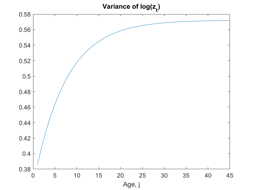
After computing the grid for log(z), Chen normalizes so that z has mean one.

Here is his Fortran code, see subroutine mchain2.f90. Note that in the subroutine he has several ways of discretizing the shocks. He chooses case 6 which is “Huggett 1996”

case(6) ! Hugget (1996)
		rho = 0.96
		sigma2eps = 0.045 ! Variance of the innovation
		sigma2y1  = 0.38  ! Variance of the initial condition eta(1) at age 1

		sigmaeps= sqrt(sigma2eps)
        ! Inputs: rho, sigmaeps, ns
		! Outputs: states (grid). stae (invariant distrib), probs (transition matrix)
        ! Width of Tauchen?? 		
		call Tauchen (states, stae, probs, rho, sigmaeps, ns)

Note that the width of Tauchen is defined inside the Tauchen subroutine. I looked in Tauchen.f90 and here is the relevant part:

! define the discrete states of the markiv chain
	
	sigy = sig/sqrt(1.0-rhot**2)

	y(n) =sqrt(n+0.0)/sqrt(2.0)*sigy
	y(1) = -y(n)

	do yc =2, n-1
		y(yc)=y(1)+(y(n)-y(1))*(yc-1.0)/(n-1.0)
	end do

It is not very explicit, but it seems that tauchen_q = sqrt(n+0.0)/sqrt(2.0) hence sqrt(7/2). Please let me know if I missed something or if you have a different interpretation

Based on this understanding, I would replace a few lines of Robert’s code with the following:

tauchenoptions=struct();

Tauchen_q=sqrt(7/2); % plus/minus two std deviations as the max/min grid points 
[z_grid,pi_z]=discretizeAR1_Tauchen(0,Params.rho_z,sqrt(Params.sigma_z_epsilon),n_z,Tauchen_q,tauchenoptions);
z_grid=exp(z_grid); % Ranges from 0.7 to 1.4
% Stationary distribution of pi_z
aux = pi_z^1000;
prob_stat = aux(1,:)';
z_mean = dot(z_grid,prob_stat);
z_grid = z_grid/z_mean;

Note that I take the sqrt of the variance and that I do the normalization

EDIT

I managed to compile and run the Fortran code and I have verified that the z_grid is correct (here “correct” means that it matches what Chen does).

aledinola · September 20, 2024, 3:51pm

Initial distribution of earnings z

Another thing I discovered going through the Fortran codes is how the paper computes the initial distribution of earnings shock z.

Basically the paper follows Huggett (1996) and assumes that log(earnings) follow an AR(1) process:

log(z_{t+1})= rho* log(z_t)+eps, where eps is ~N(0,variance)

The initial condition log(z_1) is itself a Normal random variable. Note that the variance of log(z_1) is equal to 0.38, which is lower than the unconditional variance of the process var(log(z)) = 0.045/(1-rho^2) = 0.5739. This implies that the variance of log(z_t) will increase over time as a function of t.

In my codes (which I will make available on Github) I follow Robert’s implementation but I changed a few things. For example, I discretize the initial distribution of log(z_1) using the function discretize_normal, assuming that log(z_1) has mean zero and variance equal to 0.38.

Q: Does the toolkit have a function to discretize a normal distribution with given mean and variance?

After computing the distribution of log(z_1), I assign it to the variable jequaloneDistz which is the distribution F(0 assets, 0 housing, z ,j=1)

jequaloneDistz = discretize_normal(z_grid_log,sqrt(Params.sigma_z1));

Given the distribution of log(z_1), one can then compute the distribution of log(z_t) for each t=1,..,Jr-1 using the transition matrix pi_z. All of this is exogenous, so it can be computed before solving the rest of model. I call the exogenous distribution of log(z_t) as pilab and I use pilab to compute the aggregate labor in efficiency units (also exogenous, since labor supply is exogenous). I use aggregate labor to obtain the value of pension benefits from the pension balance condition.

I compute the variance of log(z) by age, from age=1 to age=Jr-1 (i.e. only when the agent is working) and I get the following:

NOTE: the title of the figure should read as log(z_j) not log(z_t)

aledinola · September 20, 2024, 4:01pm

Grids for endogenous state variables
It turns out that grids for a and h are important to get the homeownership rate more or less reasonable. The fortran code are a bit difficult to understand but what I got is that the author defines the asset grid as equally spaced from -(1-gamma)*h to 0 and then NOT equally spaced from 0 to the upper bound, which is 100. Also, I have to use at least 300=n_a(1) to get decent results.

Transfers
In the Fortran code the transfers are given to everyone (both renters and homeowners). @robertdkirkby you have a comment in the code for this. I assume it is just a typo in the paper.

Results and open questions

After the changes outlined above, I’ve got this figure for the homeownership rate conditional on age:

The other results displayed on the screen are:

Targeted Variables 
Payroll tax rate is 0.107 
r is 6.35% 
K/Y is 2.936 
H/Y is 0.912 
Homeownership rate is 70.8% 
Nontargeted Variables 
Ho/(A+Ho) is 23.1% 
Gini for total wealth is 0.65 
Gini for financial wealth is NaN 
Gini for housing is 0.52 
Mean loan-to-value ratio (for borrowers) is NaN

Remaining questions:

Is there a toolkit function to compute life-cycle statistics by bins of say 5 years? This is what the paper does for the homeownership rate and I had to write my own function.
Not sure why the Gini for financial wealth and the LTV ratio are NaN. The lifecycle profile for financial wealth seems OK.
In my code I don’t do the general equilibrium but only a version with fixed prices.
I was able to run my code on a laptop with only 4 GB of GPU RAM. This sounds good!
The call to the function LifeCycleProfiles_FHorz_Case1 takes a long amount of time, more than the time needed to run VFI and distribution. This might be an issue if doing estimation/calibration. There are the running times in seconds (distribution is omitted since it’s super fast):

RUNNING TIMES
Time VFI: 15.749107 
Time aggvars and stats: 0.844588 
Time life profiles: 36.484752

My code is available here: GitHub - aledinola/Chen2010housing: Rough implemention of baseline model of Chen (2010) - A Life-Cycle Analysis of Social Security with Housing
Starting from Robert’s files it was easy to modify the model (many thanks to @robertdkirkby for creating the example). The difficult part was to understand the Fortran codes available on the RED website. It’s really nice that the toolkit can solve this type of models in a much easier way.

jake88 · September 21, 2024, 7:07pm

Impressive work, thanks for sharing your code! Gini coefficient NaN: generally the gini is not used for distributions that can take negative values. Here a can be nagative for home-owners.

aledinola · September 22, 2024, 8:44pm

Not sure, I think the Gini coefficient is defined also for variables with negative values (but in that case is not bounded in [0,1]).

I had a look at AllStats.A and found that the quantiles seem ok but lorenz curve is all NaN.

AllStats.A.LorenzCurve

ans =

   NaN
   NaN
   NaN
   NaN
   NaN
   NaN
   NaN
   NaN
   NaN
   NaN
   NaN
   NaN
   NaN
   NaN
   NaN
   NaN
   NaN
   NaN
   NaN
   NaN
   NaN
   NaN
   NaN
   NaN
   NaN
   NaN
   NaN
   NaN
   NaN
   NaN
   NaN
   NaN
   NaN
   NaN
   NaN
   NaN
   NaN
   NaN
   NaN
   NaN
   NaN
   NaN
   NaN
   NaN
   NaN
   NaN
   NaN
   NaN
   NaN
   NaN
   NaN
   NaN
   NaN
   NaN
   NaN
   NaN
   NaN
   NaN
   NaN
   NaN
   NaN
   NaN
   NaN
   NaN
   NaN
   NaN
   NaN
   NaN
   NaN
   NaN
   NaN
   NaN
   NaN
   NaN
   NaN
   NaN
   NaN
   NaN
   NaN
   NaN
   NaN
   NaN
   NaN
   NaN
   NaN
   NaN
   NaN
   NaN
   NaN
   NaN
   NaN
   NaN
   NaN
   NaN
   NaN
   NaN
   NaN
   NaN
   NaN
   NaN

>> AllStats.A.QuantileCutoffs

ans =

   -5.5172
         0
         0
    0.0345
    0.1225
    0.2344
    0.3723
    0.5911
    0.8359
    1.2564
    1.8754
    2.7703
    3.6629
    4.7290
    6.3294
    8.4671
   11.2955
   14.6927
   19.4442
   27.8620
   80.4070

robertdkirkby · September 22, 2024, 10:18pm

Not sure why the Gini for financial wealth and the LTV ratio are NaN.

In those results the Gini is NaN because the Lorenz Curve is NaN. This is because Lorenz Curves are not defined when there are negative values (the lorenz curve graph always starts at (0,0) and ends at (1,1), it cannot start at (0,0) if there are negative values).

There is a “Generalized Lorenz Curve” that can handle negative values (and I assume there is a Generalized Gini Coefficient you can calculate from it).

VFI Toolkit does not presently do Generalized Lorenz Curves, just plain-vanilla Lorenz Curves. Hence all the NaN.

Is there a toolkit function to compute life-cycle statistics by bins of say 5 years? This is what the paper does for the homeownership rate and I had to write my own function.

Yes, you just set simoptions.agegroupings=1:5:N_j and then use LifeCycleProfiles_FHorz_Case1. The numbers in simoptions.agegroupings are interpreted as the ‘start’ of each bin (since the above starts at 1, and then goes in steps of 5, it will give age bins of 5 model periods). Note that the default behaviour of just doing conditional on each age is essentially simoptions.agegroupings=1:1:N_j.

The call to the function LifeCycleProfiles_FHorz_Case1 takes a long amount of time, more than the time needed to run VFI and distribution. This might be an issue if doing estimation/calibration. There are the running times in seconds (distribution is omitted since it’s super fast):

That is likely almost all from the runtimes for Lorenz and Quantiles. As long as the calibration only targets things like mean you can use simoptions.whichstats to slash the runtimes during the calibration.

I will clean up the Chen codes based on what @aledinola has done sometime later this week. Thanks all for figuring out the income process and those grids!!!

General comment: this model has a perfectly elastic housing supply —you can see this as it is just ‘c+hprime’ in the budget constraint so the relative price of housing is always equal to one (unit of consumption). You could add a house price and limit the supply of housing, this would essentially just be an extra general equilibrium equation (note that currently there is no GE condition for the housing market in the codes).

aledinola · September 23, 2024, 1:53pm

Thanks a lot for your answers, Robert!

Regarding the Gini coefficient, I was able to compute it using the function lrzcurve. I don’t see how the negative values would create a problem (maybe I miss something). I have added it to my code on github.

% Gini for financial wealth
GiniA = AllStats.A.Gini;
% StationaryDist(a,h,z,j). Compute the marginal distribution of assets "a"
% and call it p
StationaryDist_a = sum(gather(StationaryDist),[2,3,4]);
[~, ~, ~, giniw] = lrzcurve(StationaryDist_a, asset_grid);
GiniA2 = giniw;

GiniA2 is equal to 0.7 more or less. The function lrzcurve is copied here:

function [pw, meanw, stdvw, giniw] = lrzcurve(p, w)

% INPUTS:
% p is the probability distrib (sum to 1)
% w is a vector with the values of the variable of interest
% (for example, the policy function for bequests/wealth)

% OUTPUTS:
% pw is a [n,2] vector with (x,y) to plot Lorenz curve

% Check if p sums to one

if ( abs(sum(p)-1)>1e-7 )
	error("Distribution p must add to one")
end


%% Eliminate elements with zero probability
p1=p; p(p1==0)  = []; w(p1==0)  = [];

%% Standard Deviation
meanw     = w'*p;
stdvw  = sqrt((w'-meanw).^2*p);

%% compute relative value for each "wealth" level
wi=p.*w; wt=sum(wi); wr=wi/wt;

%% Keep the smallest population, needed to normalize the Gini coefficient
minpop = min(p);

%% Store in a single array
pw = [p, wr, w];

%% Sort with respect to "Wealth" Per Capita
pw = sortrows(pw, 3);
pw(:, 3) = [];
pw = [zeros(1, 2); pw];

%% Cumulative p & w
pw = cumsum(pw);


%% Average bases and height for right trapezoids
height = diff(pw(:, 1));
base = (pw(1:(end - 1), 2) + pw(2:end, 2)) / 2;

% The Gini Coefficient is normalized with respect to its highest possible
% value which is obtained if the smallest population owns all the existing
% wealth.
giniw = (1 - 2 * height' * base) ./ (1 - minpop);

% plot(pw(:, 1), pw(:, 2), 'LineWidth', 4, 'Color', color);            % Lorenz Curve

jake88 · September 23, 2024, 6:22pm

@aledinola Using your function I do get the same value for the gini index, thanks. I still get nan for the loan to value ratio… any idea why is not defined?

robertdkirkby · September 24, 2024, 11:21pm

Was rereading posts above while cleaning up my codes when I saw:
@aledinola Q: Does the toolkit have a function to discretize a normal distribution with given mean and variance?
Yes, MVNormal_ProbabilitiesOnGrid() allows you to put (multivariate) normal probabilities onto a grid. Like what you did in your codes, you can also use it for log-normal probabilities on a grid just by passing log(grid) as the input. It does the ‘Tauchen approach’, in the sense it just uses the midpoints between the grid points to evaluate a (multivariate) normal cdf, and set the weights based on this; which is what Tauchen method for discretizing a markov does. [I looked at the discretize_normal() you used, and it is doing exactly this same ‘tauchen approach’, only difference being that the VFI Toolkit version can also handle multivariate normal distributions (not relevant to this model, but useful for other models).] [Currently MVNormal is the only ProbabilitesOnGrid command, but I have idea I might add some other ProbablitiesOnGrid commands for other probability distributions later.]

Also,
@jake88 I still get nan for the loan to value ratio… any idea why is not defined?
If you look at the values on grid, is one of them NaN (I am guessing that when households don’t own a house you get a divided by zero which returns NaN, and this then contaminates everything else)?

robertdkirkby · September 25, 2024, 1:23am

@aledinola your codes use n_a(2)=11 [number of points on housing grid]. Did you specifically choose this following Chen (2010) fortran codes? or was just arbitrary?