Aiyagari example, Transition

[aledinola]

I think the comments in the Aiyagari example with Transition are not consistent with the code.

The comments say that there is a change in beta (discount factor), while the code change alpha (capital share parameter in Cobb-Douglas).

As a suggestion, perhaps it would be more interesting to show a change in a tax rate, since this is the typical application of transitions in Bewley models. To keep the example simple, I would assume that there is a linear tax rate on capital income which is used to finance a lump-sum transfer. In this way, you don’t need a government budget constraint in the code.

Households budget constraint:

c + a' = (1+r_t(1-\tau))a +w_t z + T_t, \quad a'\geq 0
where \tau is the tax rate on capital income and T is the lump-sum transfer.
Implicitely, the government budget is
T_t = \tau_t r_t K_t

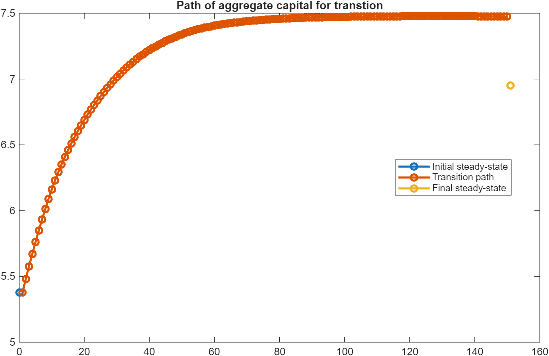
Then the experiment would be to compute the transition after the tax rate increases from, say, 20% to 40%. The code would show the evolution over time of aggregate capital, output and some measure of inequality like the Gini of assets.

This is just an idea

[aledinola]

There is a more fundamental problem. Running the transition example, I got the error about reshape gpu array

[robertdkirkby]

Infinite horizon is undergoing an overhaul. Will be some new and improved examples once done. You are absolutely right that the ‘change in alpha’ (capital share in cobb-douglas production fn) is an ‘odd’ reform.

R2025a is required for infinite horizon transition paths (because they do the Tan improvement on GPU). Deliberate decision as they had very little functionality (just transition path in Aiyagari/Pijoan-Mas), so seems fair enough that all the new functionality will require the latest Matlab. I will wait for late next year before doing all the FHorz with tan improvement on GPU, but is required for transition path in InfHorz. [R2025a is not required for the stationary general eqm in InfHorz]

[I’m guessing the error you refer to was not having R2025a, let me know if I’m wrong.]

PS. There are no ‘AllStats’ commands for transition paths yet (I will do this at some stage, for both InfHorz and FHorz, but they do not yet exist, only AggVars exists on transition paths).

[aledinola]

Great, thanks for the answer!

Gpu/reshape: yes, I ran the code using R2024b. I have R2025a already installed, so I can check but I am almost sure the error refers to not having R2025a.

AllStats: I think it’s ok not having AllStats on transition path. Once you have the policies and the agents distribution on the transition path, you can easily calculate the Gini of assets, income, etc.

[aledinola]

What is the option

transpathoptions.GEnewprice=3

?

More in detail: I would like to first try the following simple algorithm:

Start with a sequence (r_t^0,w_t^0) for t=1,..,T. Given this sequence, compute a sequence of excess demand for capital and excess demand for labor and then set the updated sequence of prices as follows:

r_t^1 = r_t^0 + 0.1(K_t^d - A_t),
w_t^1 = w_t^0 + 0.1(L_t^d - L_t^s),
for all t. Stop until the two price sequences (the one with 0 and the one with 1) are close enough.

(As you might notice, this is really not the simple Aiyagari model but a model where you need to clear both capital and labor market as e.g. in Buera and Shin 2013).

Do you think this is a decent way of implementing the shooting algorithm?

Thanks as usual!

[robertdkirkby]

transpathoptions.GEnewprice=3 is shooting-algorithm

What you have to tell it is that you want to use the GeneralEqmEqn “ExcessCapital” times “0.1” to “add” to the “r”. You do this with,

transpathoptions.GEnewprice3.howtoupdate=... % a row is: GEcondn, price, add, factor
    {'ExcessCapital','r',1,0.1}; % ExcessCapital GE condition will be negative if r is too big, so add

Similarly for the wage, so you would then have two rows, and get

transpathoptions.GEnewprice3.howtoupdate=... % a row is: GEcondn, price, add, factor
    {'ExcessCapital','r',1,0.1;...  % ExcessCapital GE condition will be negative if r is too big, so add
     'ExcessLabour','w',1,0.1};  % ExcessLabour GE condition will be negative if w is too big, so add

Setup for the GE conditions looks like

GeneralEqmEqns.ExcessCaptial=@(Kd,A) Kd-A;
GeneralEqmEqns.ExcessLabour=@(Ld,Ls) Ld-Ls;

[Kd,A,Ld,Ls are each the Mean of a FnsToEvaluate]

This is a decent way, but it’s weakness is that it is not obvious how units of the general eqm eqn K-A converts into units of r (that is, why is 0.1 a good guess?). I would normally set it up using
r^1_t=r^0_t - 0.1 (r^0_t-MPK)
where MPK is the marginal product of capital. This has the advantage that the general eqm eqn is already in units of r, rather than units of K, and so it is more obvious how much damping exactly you want/get with the 0.1. You can do them with different units for the price and the general eqm eqn, but it tends to take a lot more finessing/guessing/caressing to get update factors suitable.

---

The shooting-algorithm that VFI Toolkit uses for transition paths is based on the idea that you have n GE eqns and n GE prices. You use one GE eqn to update one price, and you do this by setting the new price equal to the old price plus-or-minus ‘damping factor’ times GE eqn. This is the info that you are encoding in how you set up transpathoptions.GEnewprice3.howtoupdate. I’m hoping to get some more sophisticated approaches to GE on transition paths, maybe later this year if I’m lucky, that will be less demanding of the user setting things up (and hopefully also just faster/cleaner).

[aledinola]

@robertdkirkby

This is a decent way, but it’s weakness is that it is not obvious how units of the general eqm eqn K-A converts into units of r (that is, why is 0.1 a good guess?). I would normally set it up using
r^1_t=r^0_t - 0.1 (r^0_t-MPK)
where MPK is the marginal product of capital

Good point. However, I am working with a model similar to Buera and Shin (2013) where there is no Cobb-Douglas production function so the condition r=MPK does not apply. The two market clearing conditions are described in your document App_BueraShin2013.pdf and shown below:

The first GE condition is what I called L_t^d=L_t^s and the second condition is K_t^d=A_t. (Actually my model is more complicated…)
In this setup I cannot use your suggestion r^1_t=r^0_t - 0.1 (r^0_t-MPK) and the tricky part is to guess the right values for the two dampening factors, which depend on the units, as you explained. Please feel free to correct me if I am wrong.

Would transpathoptions.GEnewprice=1 or 2 help? Or they are not implemented yet?

[robertdkirkby]

What you say all sounds right.

You can use transpathoptions.GEnewprice=1 but it is a bit more complicated to set up. The general eqm eqn has to be reworked so that it gives the r^{new} value directly (it is no longer a GE eqn, it is a ‘new price’ and you iterate on the transition path until ‘new price’ equals ‘old price’). Mostly it exists for legacy reasons, it was the first thing I did on the way to getting the =3 shooting-algorithm setup where the user had to hardcode the shooting update rule (=2 does not actually exist)

[aledinola]

Thanks! I found a bug in the Aiyagari transition example:

Not enough input arguments.

Error in EvalFnOnAgentDist_AggVars_Case1 (line 9)
if ~isfield(simoptions,'parallel')
            ^^^^^^^^^^
Error in Aiyagari1994TransitionPath (line 174)
AggVars_final=EvalFnOnAgentDist_AggVars_Case1(StationaryDist_final, Policy_final, FnsToEvaluate, Params, [], n_d, n_a, n_z, d_grid, a_grid, z_grid);
              ^^^^^^^^^^^^^^^^^^^^^^^^^^^^^^^^^^^^^^^^^

It is easy to fix: just add simoptions to EvalFnOnAgentDist_AggVars_Case1. it seems that simoptions is a compulsory input argument in this function. This happens on lines 113 and 132 of the main file.

[aledinola]

I ran the transition in the Aiyagari example and it converged successfully. However, there is something a little weird. I show below the transition path for aggregate capital K_t

As you can see, the transition path for K_t seems to overshoot the value of K in the final steady-state. In particular,

AggVarsPath.K.Mean(T)

ans =

          7.47352479349525

>> AggVars_final.K.Mean

ans =

          6.95178791465384

>> (AggVarsPath.K.Mean(T)-AggVars_final.K.Mean)/AggVars_final.K.Mean

ans =

        0.0750507474115592

So the difference is about 7.5 percent of the aggregate capital stock, which is not negligible.
The tolerance criterion for the transition is

transpathoptions.tolerance = 10^(-6); % default is 10^(-5)

I’m asking this question because I found the same problem in other, more complex models, with a totally different code. So probably the toolkit code is OK, but I always wondered what is going on

My understanding is that the transition path should converge to the value in the final steady-state. If not, one should either increase T or reduce the tolerance. But in this case clearly T is large enough and the tolerance is already small, so…

[aledinola]

I was looking under the hood to better understand the code for the transition and I came across the function ValueFnIter_InfHorz_TPath_SingleStep_nod_raw.

There are some inefficiencies in lines 30-34. The current code is:

EV_z=Vnext.*(ones(N_a,1,'gpuArray')*pi_z(z_c,:));
        EV_z(isnan(EV_z))=0; %multilications of -Inf with 0 gives NaN, this replaces them with zeros (as the zeros come from the transition probabilites)
        EV_z=sum(EV_z,2);

        entireRHS_z=ReturnMatrix_z+DiscountFactorParamsVec*EV_z*ones(1,N_a,1);

But it should be changed to

EV_z=Vnext.*pi_z(z_c,:);
        EV_z(isnan(EV_z))=0; %multilications of -Inf with 0 gives NaN, this replaces them with zeros (as the zeros come from the transition probabilites)
        EV_z=sum(EV_z,2);

        entireRHS_z=ReturnMatrix_z+DiscountFactorParamsVec*EV_z*;

In the first and last line, it is better to use automatic expansion.

Furthermore, since this is the branch of the conditional lowmemory=0, it would be better to eliminate completely the loop over z.

[robertdkirkby]

Is going to take me a week to two to respond. Toolkit on my computer is a bit of a mess as reworking/overhauling experienceasset to be cleaner in how it is set up internally, as well as lots of tests for it. Don’t want to go mixing that with small improvements or I might break the current github version. Hopefully will be done by end of next week and will look at this then.

[aledinola]

Thanks Robert, take your time!

[robertdkirkby]

@aledinola

I was looking under the hood to better understand the code for the transition and I came across the function ValueFnIter_InfHorz_TPath_SingleStep_nod_raw.

There are some inefficiencies in lines 30-34.

Just pushed to github cleaning this up. Nice spotting!

Will come back to answer the rest later teaching is busy at the moment

[aledinola]

Hi Robert,

I was wondering if you had any chance of looking into this problem. Just by running the Aiayagari transition example, it seems that the transition does not converge to the new steady state. Increasing T does not change the results.

Thanks a lot!

[robertdkirkby]

Not yet. Done teaching and have two weeks of code to write for coauthors. Then expecting to be doing infinite horizon transition paths all November.

[aledinola]

Thank you Rob, take your time!

A small clarification: when I say “it does not converge“ what I mean is the following: the transition algorithm does converge numerically, and the distance between successive paths for interest rate does fall below the tolerance criterion. But K(T) (or r(T), which is 1-1 related to capital) is quite different from K in the new steady-state.