I would like to build upon the setup of Buera and Shin (2013), see here, to develop a model to explain cross-country differences in TFP.
So my question is whether it is possible to replicate (and hopefully extend) Buera and Shin (2013) in the toolkit. I looked into the example of Aiayagari in the toolkit and I understand how to set the aprime,a,z variables. In my case z is entrepreneurial ability and a is of course assets. I don’t fully understand if I should add a d variable for the choice of working as a paid employeed or as an entrepreneur. Any guidance would mean a lot
1 Like
Flick me an email and I will send you an implementation of the model of Kitao (2008), which is also one of these entrepreneur-worker lucas-span-of-control setups. The toolkit solves the stationary eqm nicely, but the solution of the transition paths is a bit slow (it works, just slow). Hence why it is not yet public (in a few years with a new GPU it likely will be). That will likely give you an idea how to implement this model of Buera & Shin (2013), although as mentioned the transition paths will be a bit slow. Feel free to ask questions as you go (I have not read closely enough to know exactly what is different in the two setups).
The worker-entrepreneur is handled as a two-valued endogenous state, and the contents of the return function then just involves a big ‘if’ statement depending on which of the two the agent currently is.
[There is a computational trick that I can use on the stationary model, but which doesn’t work in transition, and is nice for this kind of model. Hence the difference (called ‘refine’ by the toolkit, it is on by default)]
1 Like
Hi @javier_fernan, great question. I think I have some old files where I attempted a replication of this paper (back then I did not know how to implement this model using VFI toolkit). Now, thanks to Robert’s very nice explanation, I know how and I might do it in the future when I find a bit of time.
One suggestion besides what Robert wrote: You can easily compute k, \ell (the demand for capital and labor by entrepreneurs) and the profit \pi analytically and write the equations in the ReturnFn. This should speed up the code a lot and even allow for the transition. Of course if you want to extend the model, these closed form results may not be available anymore ![]()
1 Like
Cool! If the closed forms work then the toolkit should easily handle what is left as it will just be a single endogenous state.
I went and actually read the paper last night. Turns out Buera & Shin (2013) at a strictly computational level is a transition path in a model with one endogenous state and two exogenous states. So I spent the morning implementing it and here it is (code and a pdf; runs on my desktop GPU with 8gb GDDR):
Key to all of this is that the firm problem is static, and so is the entrepreneur/worker decision problem. (Unlike what my above post was guessing would be the case).
A few comments:
(i) I call entrepreneurial ability z (BS2013 call it e)
(ii) I had to use three exogenous states (z,tau,psi_v). The reason is that tau transitions iff z transitions, and to impose this I needed to add in psi_v (psi_v is essentially just reflecting the probability psi). BS2013 would not have needed this because they could have just hardcoded the ‘iff’.
(iii) I had to change the value of beta (BS2013 use 0.904, but this gave me a negative interest rate, so I change it arbitrarily to 0.8) [to know why would require the codes of BS2013, if I planned a full replication I would ask them for the codes, but I don’t presently plan to complete a replication]
(iv) I have not checked how many asset grid points are appropriate, I may have too many (which slows code down) or I may have too few (which would be inaccurate). I am probably ballpark okay but really you should run it a few times with different number of points and find a good speed/accuracy balance.
Lastly, Javier, since you wanted to get into this model, I would be very grateful if you can please double check my algebra in the pdf (replacing the firm profit maximization problem with analytical values for k, l and pi). There were a lot of exponents flying around so it is totally plausible I made a typo error.
[I will likely update the code in the next few days to add a few graphs of the transition path results]
[As ever, a caveat that writing code dedicated to this model would give faster runtimes]
1 Like
Just to mention the transitions are not actually working yet (it is the code, not just you ![]() )
)
I think I have an idea what I got wrong, but don’t have time to try fix it right now, hopefully next week.
(code is fine for stationary eqm, is just the transition path that is not yet smooth)
I apologize for the long delay, finally I managed to come back to this project. Thanks @robertdkirkby and @aledinola for your replies!
I downloaded the files from dropbox, but when I run the code buerashin2013 I get an error
Error using gpuArray/arrayfun
Maximum variable size allowed on the device is exceeded.
Error in CreateReturnFnMatrix_Case1_Disc_Par2 (line 100)
Fmatrix=arrayfun(ReturnFn, aprime1vals, a1vals, z1vals,z2vals,z3vals, ParamCell{:});
I think my laptop does not have a good memory. Can you please instruct me on how to solve this issue? I tried to reduce the number of points on the grid but then the general equilibrium does not converge.
P.S. @robertdkirkby I read your pdf and I didn’t find errors. I thanks you again for the time that yopu spent on this
@javier_fernan you could try the option
vfoptions.lowmemory=1
This will reduce the amount of RAM needed but the code will be slower
1 Like
Error using gpuArray/arrayfun
Maximum variable size allowed on the device is exceeded.
This is essentially saying that there is not enough GPU memory to create that big of a matrix. There are three ways to ‘solve’ it. One is to buy a new GPU with more memory (obviously not exactly an easy fix). The other is to use smaller grids (although as you note this could be problematic as not accurate enough). The third is what Alessandro mentioned about vfoptions.lowmemory=1 which uses more loops (so runs slower, but uses less memory).
Note that it is GPU memory, not standard CPU memory that has run out. (GPUs have their own GDDR memory, which is typically a much smaller number of gigabytes than you will have of CPU memory.)
2 Likes
Thanks! I will try with vfoptions.lowmemory=1
Ok, I tried vfoptions.lowmemory=1 but is really slow… it takes forever to compute an equilibrium. With smaller grid the running time is fine but the equilibrium does not converge. I will try to get a new computer at some point in the future but it won’t be soon. In the meantime, is there any other option that I could try?
Sorry but no.
Obviously it is possible to solve it faster, just not with VFI toolkit. The toolkit does not use the algorithms with the best speed-accuracy trade-off. Instead it uses algorithms with a decent speed-accuracy trade-off, but which can be implemented in a very general and robust, easy-to-use way.
2 Likes
Got it, thank you so much for all the help!
1 Like
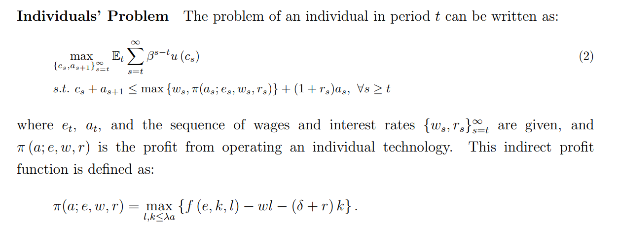
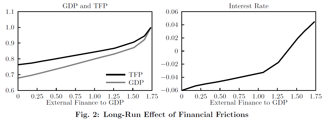
I went back to your nice example of BS2013, Robert. I simplified the model in the sense that I focus only on the steady-state, with the aim or replicating Figure 2 of the paper. The figure shows the impact of financial frictions on interest rate, GDP and TFP, starting from the benchmark economy calibrated to the US with lambda=inf.
The benchmark is an economy without financial frictions. There, the external finance to GDP ratio is 1.75 and the equilibrium interest rate is 4% (see right panel). GDP is normalized to 1 in the left panel. I think in your example you set lambda = 1.35 and this is why you don’t get the 4% equilibrium interest rate with beta=0.9.
As you lower lambda from inf down to 1 (which means that external finance/GDP drops from 1.75 to 0), you reduce demand of capital by entrepreneurs and increase savings (b/c the entre need to self-finance their business) so the equilibrium interest rate must fall. In the economy with lambda=1 you get r = - 6%. In this setup, negative values of the interest rate are totally fine (I think). We don’t have a CRS production function that pins down r and w.
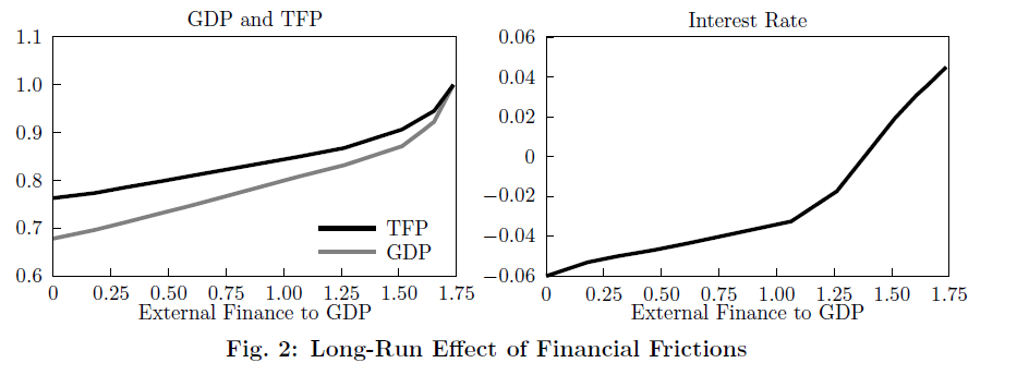
I have a forked repo on my github that replicates the steady-state of BS2013 and then computes a sequence of steady-states to generate Figure 2 of their paper. My replication of their figure is this:
Note that I do not plot TFP in the left panel but only GDP (I didn’t understand how BS compute TFP in their model)
Overall, thank you so much Robert for providing this example! It was relatively fast to build on your codes. I conclude with three technical observations:
- I decreased the number of grid points from 1501 (Robert’s codes) to 1001 and didn’t have any convergence problem.
- As I wrote in (1), convergence is not an issue even with fewer grid points, but GE loop is slow. To speed it up a bit, I loosened the tolerance criterion for fminsearch from 1e-4 to 1e-3. Thanks @robertdkirkby for implementing this feature a while ago.
- I got rid of the exog state psi: I only use z as a single exogenous Markov state. The trick is this: if today’s ability is z(i), then tomorrow’s ability will be z(i) with
prob=(1-psi)+psi*p(i)and z(j) withprob=psi*p(j)when j~=i. The vectorp=pi_z_vecdenotes the probability mass function of the discretized Pareto shock. Then you can build the transition matrixpi_z(z,z')with the following line of code:
pi_z = Params.psi*eye(n_z)+(1-Params.psi)*ones(n_z,1)*pi_z_vec';
1 Like
As a final thought on the economics of the paper: BS2013 claim that they can explain well stylized cross-country evidence. This is true for GDP and TFP but much less so for the interest rate: in their model, developing countries with high financial frictions (so lambda close to 1) have negative real interest rate, while in the data is just the opposite. Of course this is because their model has just one ingredient and misses other aspects important for developing economies like default etc
1 Like
Those Figures look nice ![]()
The change to include psi at part of a one-dimensional z is a good idea! I might go change my version of the codes to incorporate that.
1 Like
One trick that turned out to be useful when solving for several steady-state while varying lambda:
for ii=1:length(lambda_vec)

    %Assign lambda:
    Params.lambda = lambda_vec(ii);
    % Solve model and store equilibrium r and w
    % in r_vec and w_vec
    % [....]

     if ii==1
        Params.r = 0.0472;
        Params.w = 0.171;
    elseif ii>1
        Params.r = r_vec(ii-1) ;
        Params.w = w_vec(ii-1);
    end

end
So what I do is first to find a decent initial condition for r and w for the first steady-state, corresponding to ii=1. Then the initial conditions for ii=2 is the equilibrium for ii=1 and so on. This strategy relies on the property that the equilibrium values of the prices r and w vary smoothly with respect to lambda.
Another thing I wanted to check: since fminsearch is a bit slow, maybe fsolve is faster (this is a TODO for whenever I find time to go back to this)
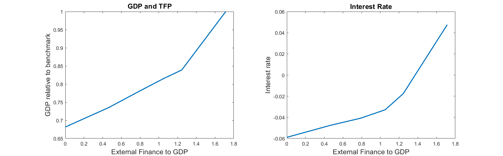
I’ve completed the replication of the steady-state of Buera-Moll (2013). In particular, I have replicated the calibration of the steady-state in Table 1.
Original table from the paper:
My table:
 \begin{tabular}{lcc} \hline
  & US Data & Model \\
 \hline
Top 10 Employment        &    0.670 &    0.658 \\
Top 5 Earnings           &    0.300 &    0.369 \\
Establisments exit rate  &    0.100 &    0.100 \\
Real interest rate       &    0.045 &    0.048 \\
\hline
 \end{tabular}
The only visible discrepancy is in the top 5% share of earnings: BS2013 match exactly the data value of 30%, while I get 36.9%
Figure 2 (original vs replication)
General comments on the replication:
(1) At least for the steady-state, everything replicates well
(2) The discretization of the z shock is not very well explained in the paper
(3) Not explained how to compute aggregate TFP
(4) Code for VFI and distribution is fast, but it takes time to find the general equilibrium. fminsearch does not converge if the initial conditions are not chosen carefully.
(5) I computed the exit rate myself in the function fun_entry_exit (here) because it would have been too complicated with the toolkit. Now I define the state space as (a,z). If instead I define the state space as (a,e,z) where e is a dummy variable (1=entrepreneur and 0=worker) then the exit rate can be computed as
FnsToEvaluate.Exit = @(aprime,eprime,a,z) e*(1-eprime);
AllStats.Exit.Mean
This means e=1 today and eprime=0 tomorrow.
1 Like