Deadbeat agents and feasibility constraints

In my model, agents don’t earn enough to cover expenses when they are young (kappa_j too small early in life), but as they gain experience and earning power, they can pay off their debts and buy houses instead of renting. And I have this working, but it is fragile, due to this constraint:

net_worth_prime=aprime+hprime;
if agej<11
    if net_worth_prime<-debt_limit*(11-agej)/10
        % Limit starter loan needed to get people going
        return
    end
end

In the first year, they max out their debt (debt_limit). But then what I want them to do is to retire a fraction of that debt every year until year 10, when such starter loans are no longer offered. debt_limit is enforced by the grid, so it is impossible to borrow more than that.

What seems to happen is that when agents’ earnings are marginal, they max out their debts and stay maxed out, leading to a financial dead-end in the Policy states (labor allocation is zero and they are stuck).

If instead I add a large negative value, say -20, to the return function, then the policy iterations discover this is disfavored and instead plot a course of sensible debt repayment.

I believe that the behavioral difference between a highly disfavored solution and a forbidden one is telling me that I actually have not conditioned my problem well in the first place. Imaging that the consumption function c has various labor-related things added and various living expenses subtracted, we then account for the assets a which may be negative or positive:

if a<0
    % Subtract loan interest by adding diminishing assets
    c=c+(1+r_r_wedge)*a-aprime;
else
    % Deposit interest included in augmented assets
    c=c+(1+r)*a-aprime;
end

Looking at the above, if the agent is big in debt (negative a), and she wants to keep c above zero, she needs to subtract a correspondingly high negative aprime, which keeps her in debt.

If I penalize the debt in the return function, a viable solution is found. If I forbid the debt, there’s no escape. Is my mistake with respect to using the periods used for the values in my debt calculation, or are there other limitations as to when one can or cannot forbid certain choices?
Mathematically there is no reason why there cannot be points from which it is impossible to financially recover (if you live 20 periods, have income of 2 each period, and start with debt of 100, it is impossible to recover if there is no bankruptcy to allow you to escape debt).

So your model is giving the ‘correct’ answer to the setup you have given it. If you don’t like the answer, it is likely that you didn’t get something about the setup ‘correct’ with how you are thinking about it.

[If people get into a situation where the return fn is -Inf, then they will ‘give up’.]

PS. In any model where income is hump-shaped, consumption-smoothing means young people will borrow (so as to smooth their consumption). My guess if that you have this motive already, and then presumably added another motive, making debt super tempting to them. Your comment that

If instead I add a large negative value, say -20, to the return function, then the policy iterations discover this is disfavored and instead plot a course of sensible debt repayment.

suggests something like this. Your model currently has debt being super tempting for some reason.

It was beta! A beta<1 provides incentives to take on more debt, while beta>1 helps the agents buy investments. There are obviously many ways to skin this cat, but this was particularly simple (and harmonious to other things I’m doing).

I’m continuing my exploration here, and realizing that LifeCycleModel35 does not charge interest on loans. I’m still working on letting the math speak and not writing too many conditional guidance terms in the return function, so I’m still trying to figure out all to allocate the interest payment across the consumption function elements (F, c, aprime, hprime, not to mention leisure, etc.).

I know that bank officers look at not only debt-to-equity ratios, but also debt-to-income ratios. I’m looking to create the most elegant return value F, meaning the least conditionalized function of consumption, housing services, savings, etc. that results in the agent making both maximizing and prudent decisions about when to buy or sell houses, with what amounts of debt, at each age in their uncertain lives.

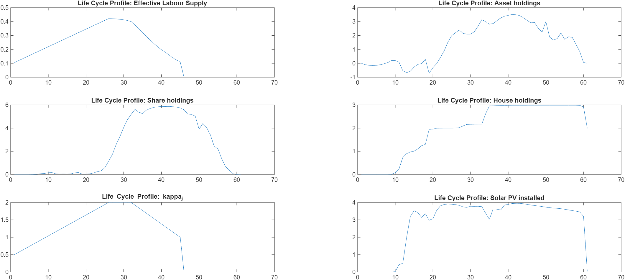
My agents are now making sensible decisions, buying larger houses as they grow in earnings power and wealth. With SolarPV to offset ever-growing energy costs. I probably need to increase the scale on some of the grids, but it’s all starting to work now!

1 Like

I want to better understand what happens when my agents are bankrupt.

Under one set of economic parameters, which has both z and e shocks, the agents skate close to the edge (notice the minimum in the 3rd period):

Minimum: [0.054372    0.015388    0.00020512    0.10557    0.074656    0.081082    0.10795    0.14754    0.1498    0.15382    0.22123    0.4089    0.47108    0.7128    0.78848    1.0051    1.1135    1.806    1.6642    1.7741    …    ]
Maximum: [0.0543721    0.332888    0.45859    0.582182    0.847156    0.896875    0.864008    1.02473    1.0292    1.22567    1.64299    2.11332    2.48213    2.91731    3.81352    5.07812    5.73864    8.24    7.05014    7.6737    …    ]

If I change one parameter (energy cost) just a little bit, some agents cannot meet their consumption requirements (if you scroll to the right, you’ll see they eventually do recover):

Minimum: [0.028772    0.0073068    -1.1136    -1.1552    -1.194    -1.2304    -1.2648    -1.2975    -1.3288    -1.3588    -1.3877    -1.4155    0.0071757    0.19555    0.19409    0.21803    0.43382    0.69086    0.86809    1.0041    …    ]
Maximum: [0.0287721    0.634412    0.713938    0.556582    0.931548    0.979073    0.899296    0.999127    1.06487    1.22244    1.64239    2.06152    2.62933    3.0645    4.09021    5.06532    5.73224    8.1184    7.04374    …    ]

One statistic I could collect is the collective negative consumption of a given time period, which could inform how much public benefit we may need to pay so that shocked agents can pay their bills as they fall due. That could function as a kind of exogenous disruption to the balancing of the Government Budget, forcing the equilibrium solver to properly allocate that amount via an increase in payroll taxes.

But the question that’s vexing me now is this: when negative consumption leads to infeasibility for the return function (-Inf), what, really, happens to the agents? Do they evaporate from the total agent mass, reappearing when the solution is no longer infeasible? And if they reappear, what happened to their assets, their houses, their cars, etc? If they don’t disappear, how are they counted among the general statistics? And what are the implications of the direction of our iteration (forward or backward) in the case of appearing and disappearing?

In terms of the code they are still there, but they are just going to act in a stupid manner.

Essentially, you should always avoid anything that returns -Inf, because the problem is not well defined in that region.

[stupid manner=choose the first grid point, as that is Matlab’s default answer to max of a vector of identical numbers]

The -Inf return value is usually where things are very marginal: z and e both against the agent. When you say “avoid the region” does that mean just the matrix points affected, or all the z and e points that sum together I’d the d, aprime, a plane?

Unless they all leave that area next period, include all the z and e dimension. But if they leave next period you don’t need to worry about the other z and e.

[The rest of the z and e will not matter to ReturnFn, but they will contaminate the expected next period value fn]

Returning to this thread because I’m again thinking about reporting what percentage of agents are living in the infeasible region. I think the answer to my question is this: presuming I set up the grids to that Policy State 1 is an infeasible state (and thus the collector of all infeasible states based on the behavior of the max function), I can calculate the percentage of agents alive but not part of the meaningful means, minimums, and maximums by calculating the age weights of State 1. Is that correct? If so, then I can also calculate the percentage of agents either leaving or entering the “real” model on a period-by-period basis, which would be grand.

To record and query the history of State 1 occupancy, from the State 1 perspective, it seems like CustomModelStats is the way to go: define a J-sized array as part of Parameters and at each age going forward, calculate the percentage of State 1 agents.

But if we want the agents view of their history, that sounds like something we can only calculate using the simulation panels, with each agent recording their own history. I don’t see an easy way for a cohort of agents who all wind up in State 1 at age J to discern whether they all got there because of the same misfortunes they all share, or misfortunes unique to themselves. There might be a middle ground whereby an agent history is recorded as the number of times they hit the screen. In which case we don’t need one array per agent, but at most a JxJ matrix where the row rank is the count of historical misfortunes, the column is the age, and the column value is the percentage at this age in State 1. The most unfortunate agent of all is one who has been in State 1 through the whole model, leaving a trail of percentages along the diagonal of the matrix.

Might there be an interesting way of using an ExpAsset to track recent, cumulative, and/or historical State 1 occupation on an agent-by-agent basis (letting probabilities, not simulation) do the work for us?

Easiest would be a simulation and looking at agents. In principle you could use transition probabilities to understand what is the probability given that you are now in your present state, that you got there by coming from state X. But if you want a yes/no answer to coming from state X this would have to be done on an individual simulation basis.