Example: Attanasio, Low & Sanchez-Marcos (2008)

[robertdkirkby]

Just uploaded codes implementing Attanasio, Low & Sanchez-Marcos (2008) - Explaining Changes in Female Labor Supply in a Life-Cycle Model

Codes and pdf of model: https://github.com/robertdkirkby/LifeCycleOLGReadingList/tree/main/AttanasioLowSanchezMarcos2008

Comments:
i) paper is a bit messy on equations and parameters, so not 100% sure parameters are all correct in my codes
ii) model has bivariate joint-unit root, you should renormalize model to remove this from state space, but I just discretize it and solve. Means code is solving a ‘harder’ problem, but also makes it easy to change to any other process on earnings shocks.
iii) results differ from ALSM2008, main direction is always the same but, e.g., ALSM2008 report that 47% of women with children under 3 work, while here codes say 2%. [look at Figure 10 in paper and code and you can see the shape is identical, just the magnitude is very different]
iv) decent odds that (iii) relates to (i) [of course maybe there is just a mistake in my code, but I can’t see it, or maybe there is error in ALSM2008 original code]
v) behaviour of assets in model is very unrealistic, this may also be related to (i), ALSM2008 do not report any results relating to assets, so not sure if theirs looked more reasonable. That said, this is a model without retirement (nor a warm glow target level of assets to substitute for it) so the asset profile may well just be supposed to look this way.

This example shows two things in toolkit not yet seen elsewhere. One is discretizing a life-cycle VAR(1), second is ‘experienceasset’ which is used to model the ‘history of female labor force participation’ (h_f in model). ‘experienceasset’ can be used for many kinds of human capital models and will get properly documented sometime late next year.

[Requires a fairly powerful gpu to run as is, but if you just want to play with it then make the grids smaller and will be fine on standard desktop gpu. Even with grids half the size I got same results.]
[The original fortran codes and data work are available on Low’s website]

[aledinola]

The new feature of the toolkit “experienceasset” is great! I managed to set up a simpler version of ALSM (2008) while preserving the main features of the model:

• Married couples with female labor force participation decision {0,1}
• Consumption and savings
• Human capital of women: goes up if labor supply = 1, depreciates at rate delta is labor supply is 0. The law of motion of human capital is simple:

h_f_prime = G(h_f,l_f,age)
where h_f is human capital and l_f is labor supply (either 0 or 1)

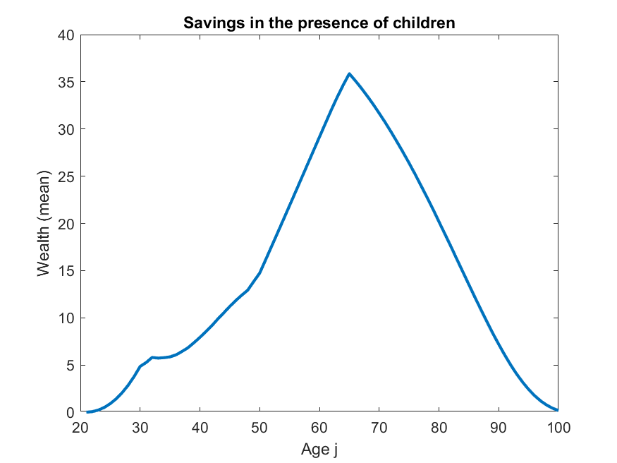
The code runs reasonably fast. The income and labor force participation profiles look good but I suspect that there is some problem with assets. The asset profile and the distribution are strange. As a test, I impose that human capital stays constant at one (so this goes back to a one-asset model) and still the weird result about asset remains. Whenever I have time I will share my simple example here and/or on Github.

[robertdkirkby]

Can you please email me a copy of your codes so I can take a look, try debug.

[aledinola]

Sure, I’ll send you an email. To quickly explain what I did, I have a relatively simple model, summarized in the Return Function and the function for human capital accumulation

function F = f_ReturnFn(l_f,aprime,a,h_f,eta_m,eta_f,theta,w_m,eff_j,w_f,...
    pchild_j,pen_j,r,nchild_j,crra,nu,agej,Jr)

F = -inf;

% Calculate earnings (incl. child care costs) of men and women
y_m = w_m*eff_j*theta*eta_m;
y_f = w_f*l_f*(exp(h_f)*theta*eta_f - pchild_j);
% l_f can be either 0 or 1
% calculate available resources
cash = (1+r)*a + pen_j + (y_m + y_f)*(agej<Jr);
cons = cash-aprime;

if cons>0
    F = (cons/sqrt(2+nchild_j))^(1-crra)/(1-crra) - nu*l_f;
end

end %end function "f_ReturnFn"

Please note that in f_HC_accum I have imposed h_f_prime=h_f to debug, but you can revert to the original case.

function [h_f_prime] = f_HC_accum(l_f,h_f,age_j,xi_1,xi_2,del_h,h_l)
% l_f: d variable that affects h'
% h_f: current-period value of h

%h_f_prime = h_f + (xi_1 + xi_2*age_j)*l_f - del_h*(1-l_f);
%h_f_prime = max(h_f_prime, h_l);

h_f_prime = h_f;
%h_f_prime = max(h_f_prime, h_l);


end %end function

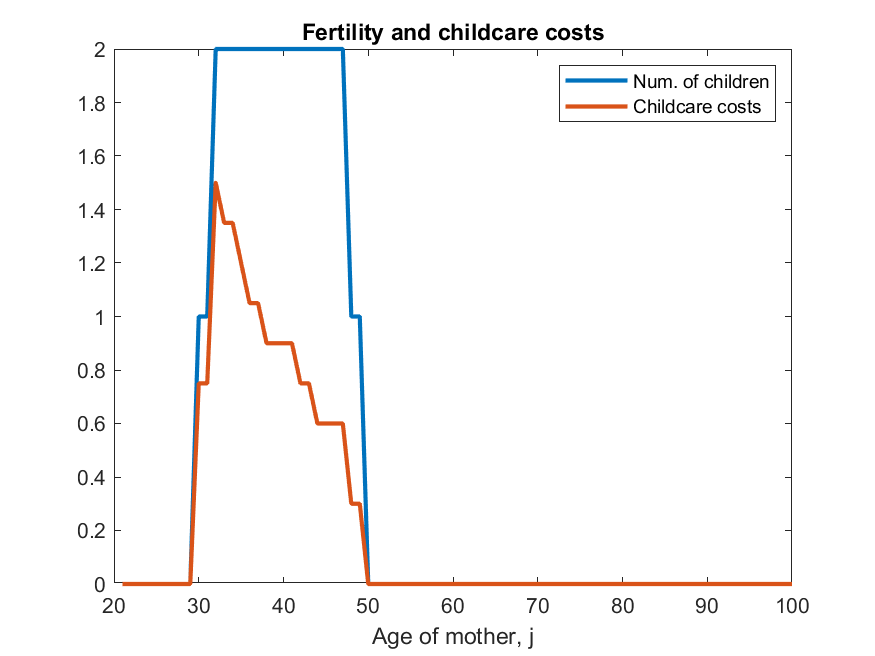
The age-dependent parameters nchild_j and pchild_j denote the number of children and the cost of childcare, respectively (conditional on age, all households have the same number and age of children) and are plotted below:

So basically women have two children around age 30, children stay in the household until they are 18 years old and older children generate less childcare costs.
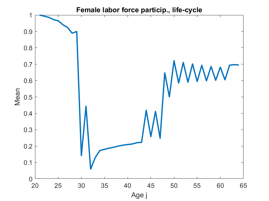
This is the life-cycle profile of labor force participation:

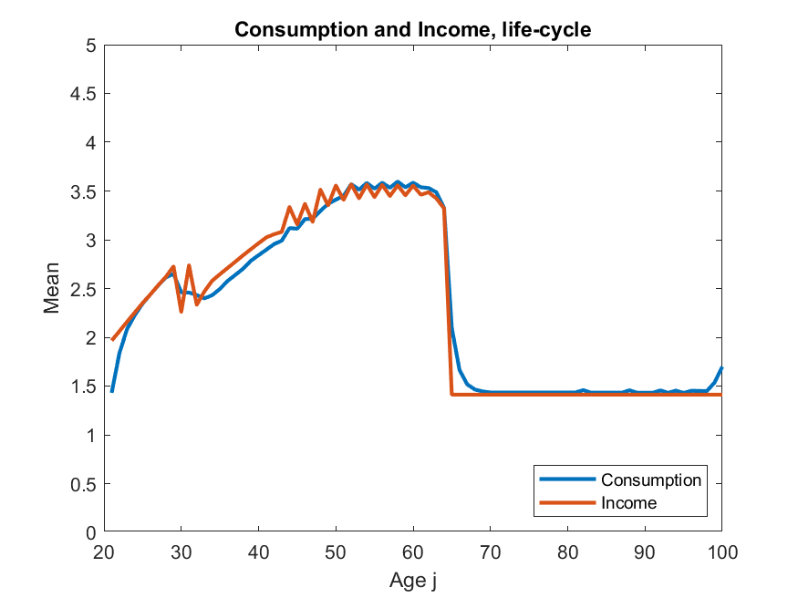
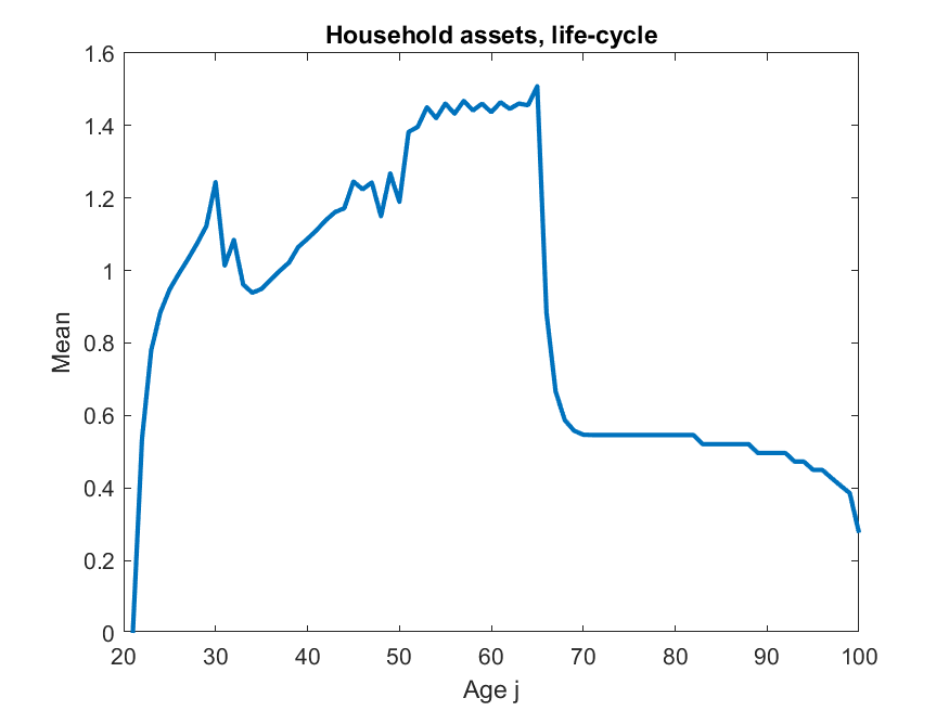
which seems reasonable (note the drop in LFP when children arrive). But the profile of consumption and asset holdings don’t make much sense

From the figures it is evident that households save too little and basically consumption tracks income. To debug, I make sure that the lifecycle profile of human capital for women is always at one, so that you can solve the model without using experience assets. If you solve the model without experience assets, the results are different but make sense.

[robertdkirkby]

I’ve discovered and fixed the issue, but will take me a day or three to roll it out across all the experienceasset codes (rather than just the specific combo this was using). I’ll let you know once it is all pushed to github.

[When I first wrote them I was trying to be tricky, using kron() in high-dimensions as it can be tiny-fractions of a second faster that repelem() and repmat(). But it was too tricky, and I got some dimension orderings confused. On the plus side, while fixing this, I realised there was a cleaner and better way to handle the interpolation step, in terms of when I do that step, so it everything will be nicer now.]

[aledinola]

Great, thanks a lot!
It would be nice to add this case to the pseudocodes document, for future reference.

[robertdkirkby]

It would be nice to add this case to the pseudocodes document, for future reference.

Just human capital (experienceasset), or you mean also with another endogenous state?

[aledinola]

Just human capital, say h’=G(d,h) where G(.) is the law of motion of human capital, h is today’s human capital and h’ is tomorrow’s human capital and then d is a choice variable (e.g. labor supply) that affects human capital. This should cover ALSM (2008).

[robertdkirkby]

Codes are all fixed (they are much nicer and better now, I’m actually happy with them for the first time which means they will become publicly documented soon, maybe next month; I did both experienceasset and also the no-where-yet-mentioned experienceassetu which does uncertain human capital).

I also updated the pseudo-codes to explain experienceasset, which does aprime(d,a). Main trick is that I replace next-period V(aprime) with V(d,a) by linearly interpolating aprime(d,a) onto the grid on a.

vfitoolkit/Pseudocodes/blob/main/VFI_PseudoCodes.pdf

[aledinola]

This looks great, many thanks for your effort!

I have downloaded the new codes and ran the simple model. Now the life-cycle profiles make sense (also for assets) but I suspect there might be something wrong still, in particular for the d variable (in this case, female labor force participation, 0-1).

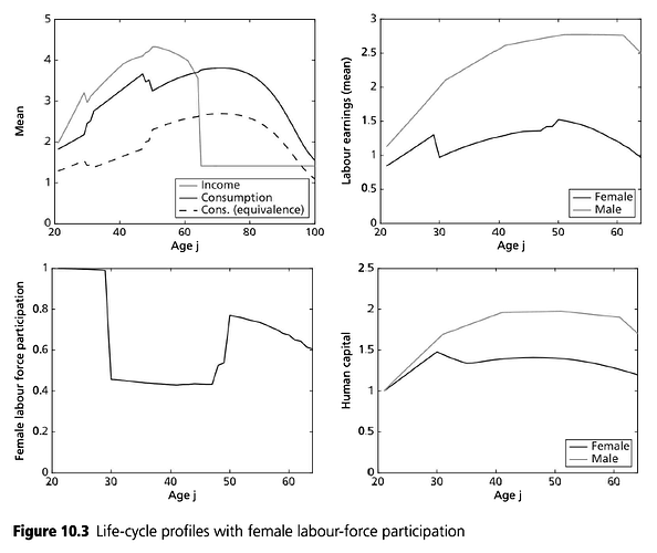
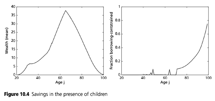
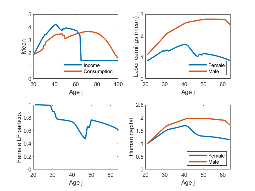
The example is actually taken from the textbook of Fehr and Kindermann ( Introduction to Computational Economics Using Fortran, pp. 429-444). They provide the Fortran codes, with parameter values and everything here. The results are the following

and here is my (partial) replication with the VFI toolkit:

I am quite confident that the results in the book are correct since I rewrote the Fortran codes from scratch myself and I got very similar results. The replication based on the toolkit, however, has a strange discrepancy in (i) female labor force particpation and (ii) female human capital. Here is why I think the toolkit results are not correct: households have children at ages 30 and 32, so many women drop out of the labor force around that age. Human capital of women takes a hit around age 30-32, goes down a bit and then recovers. In the toolkit results, instead, there is a larger drop around age 40-45 that is difficult to explain.
Also, the toolkit almost perfectly reproduces the asset results now (a1 in the toolkit notation), which makes me think that there could be some problem with the d variable, and with a2 (which is human capital).

Of course, as always with these replications, there might be a bug in my codes Another possibility is that the algorithm makes a difference: Fehr and Kindermann’s Fortran codes do VFI with linear interpolation also on a' (and a' is chosen using Brent’s method). I tend to discard this last possibility, though, since FK use 80 grid points for assets while I use 600 points with the toolkit, so it’s not an accuracy issue.

All in all, I think that this example about dual earners and human capital accumulation, borrowed from Fehr and Kindermann’s textbook, can be a useful way to test this new feature of the toolkit (experienceasset). If you think it is a good idea, we can coauthor a replication of this example and add it to your document on the Intro to life-cycle models.

P.S. To generate the new figures, I have put human capital accumulation back in the model:

function [h_f_prime] = f_HC_accum(l_f,h_f,age_j,xi_1,xi_2,del_h,h_l)
% l_f: d variable that affects h'
% h_f: current-period value of h

h_f_prime = h_f + (xi_1 + xi_2*age_j)*l_f - del_h*(1-l_f);
h_f_prime = max(h_f_prime, h_l);

%h_f_prime = h_f;
%h_f_prime = max(h_f_prime, h_l);


end %end function

[aledinola]

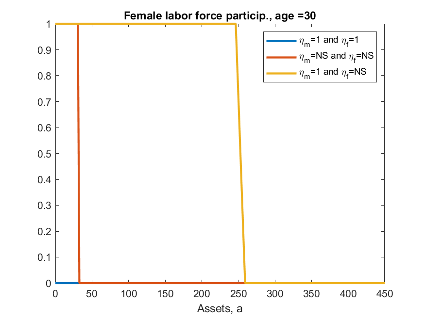
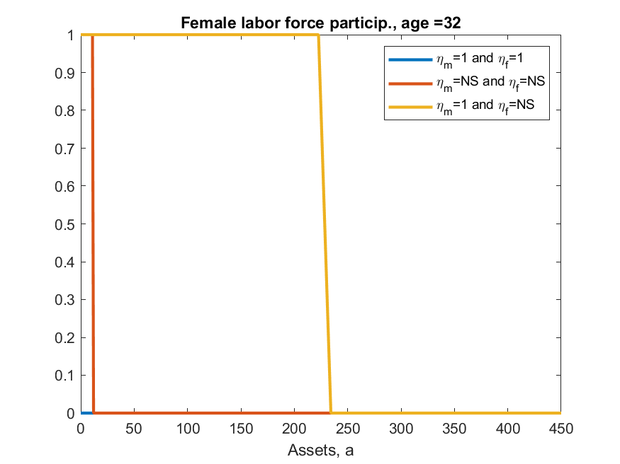
I attach here some policy functions, based on the Fortran code

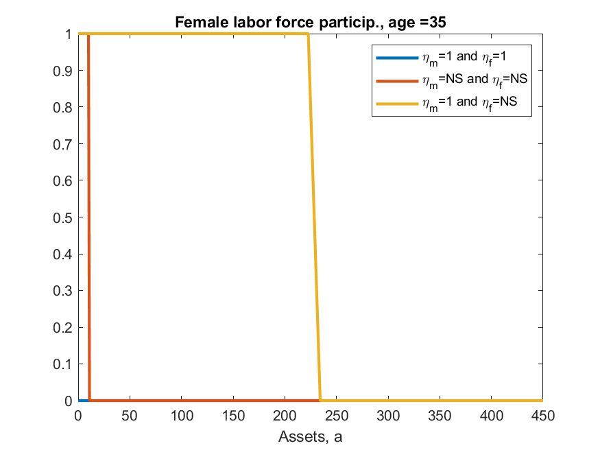
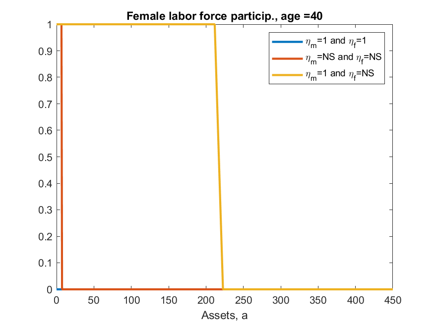
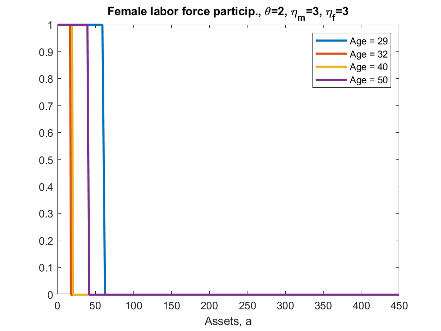
The last figure plots the policy function for female labor supply, l_f, as a function of assets, for given values of the exogenous shocks (eta_m=3,eta_f=3,theta=2) and for different ages. You can see that from age=29 to age 32, many women go from l_f=1 to l_f=0 (Note that most of the distribution is concentrated at asset levels below 100). Then at age 50 many of them come back to work. This is consistent with the life-cycle profile of female labor supply.

Unless otherwise stated, I always fix theta=2 (i.e. I set the permanent type to college-educated).

Last thing: age in the code goes from 1 to 80 but the age shown in the plots goes from 21 to 100 (since households enter the model at age 20)

[aledinola]

I’ve read the pseudocodes, new section on experienceasset. All clear, apart from

Evaluate aprime(a, z) on the grids for a and z

But aprime depends on (d,a), not on (a,z), correct? Therefore there should also be a loop over d when creating the EV term

[robertdkirkby]

Should have been aprime(d,a) right through. Fixed now. Thanks for pointing that out

[aledinola]

I double coded the model in matlab to compare the toolkit vs another solution based on discrete vfi and I found perhaps surprisingly that the discrepancy is the distribution. If I replace the toolkit codes with my customized code for the distribution I can replicate roughly the Fortran results (roughly because the Fortran codes use a different solution algorithm)

I want to have another look at my code (hopefully I should have time this week) and then I’m happy to share it

[robertdkirkby]

Found and fixed one thing (when trying to leave grid, I was handling bottom of grid fine, but not top of grid). Let me know if there is still issue with the stationary dist.

[aledinola]

Great, thanks! Now the results are consistent with my customized codes

Can you please point out at the functions that you have updated? (I can also have a look at github…)

UPDATE:
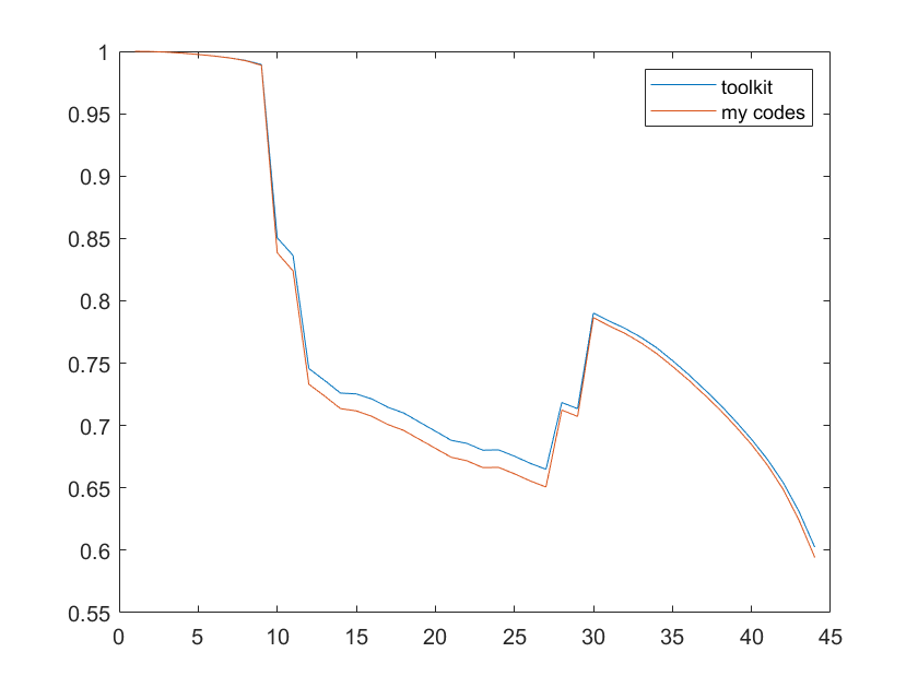
There is still a very small difference b/w the toolkit and my codes in the Distribution. Policy functions are identical

||Policy_toolkit-Policy_ale||

 0

||StationatDist_toolkit-StationaryDist_ale || =

  0.000538689835730402

And the life-cycle profile of d (i.e. female labor force participation) is now very close (before it was really different)

As a side note, I did not understand exactly what is the problem here:

% Precompute
II2=[1:1:N_a*N_z; 1:1:N_a*N_z]'; % Index for this period (a,z), note the 2 copies

for jj=1:(N_j-1)

    % First, get Gamma
    Gammatranspose=sparse(Policy_aprimez(:,:,jj),II2,PolicyProbs(:,:,jj),N_a*N_z,N_a*N_z); % Note: sparse() will accumulate at repeated indices [only relevant at grid end points]

I would simply treat the left and right points separately

% Precompute
%II2=[1:1:N_a*N_z; 1:1:N_a*N_z]'; % Index for this period (a,z), note the 2 copies
II1=(1:1:N_a*N_z)'; 

for jj=1:(N_j-1)

    % First, get Gamma
    %Gammatranspose=sparse(Policy_aprimez(:,:,jj),II2,PolicyProbs(:,:,jj),N_a*N_z,N_a*N_z); % Note: sparse() will accumulate at repeated indices [only relevant at grid end points]
    Gammatranspose=sparse(Policy_aprimez(:,1,jj),II1,PolicyProbs(:,1,jj),N_a*N_z,N_a*N_z)+...
        sparse(Policy_aprimez(:,2,jj),II1,PolicyProbs(:,2,jj),N_a*N_z,N_a*N_z);

This does not solve the discrepancy but it is faster and less memory intensive. I opened an issue on Github: Issues · vfitoolkit/VFIToolkit-matlab · GitHub

My files are available here: GitHub - aledinola/ExperienceAssetAle

In main.m, see flag do_toolkit. If equal to 0, runs my codes, if equal to 1 runs the toolkit codes. This makes it easy to compare the two. To make the comparison, run test.m

P.S. I am not so sure anymore about the Fortran codes

[robertdkirkby]

The fix was in the code that takes Policy and figures out the upper and lower grid points (and their probabilities)

vfitoolkit/VFIToolkit-matlab/blob/master/aprimeFnMatrix/CreateaprimePolicyExperienceAsset_Case1.m

Specifically, around line 127 I do,
[~,a2primeIndexes]=max((expasset_grid>a2primeVals),[],1);
which is to find the first grid point larger than a2primeVals (the upper grid point), where a2primeVals is the value of the policy that I want to put onto the expasset_grid.

Problem, which I now know but did not previously realize, was that this works for everything except when a2primeVals is bigger than all grid points (it does work for a2primeVals is smaller than all grid points). So I have just had to add a line later to deal with the case where a2primeVals tries to leave the top of the grid, namely I sort out trying to leave top and bottom of grid with lines

% Those points which tried to leave the top of the grid have probability 0 of the lower point (1 of the 'upper' point)
offTopOfGrid=(a2primeVals>=expasset_grid(end));
a2primeIndexes(offTopOfGrid)=n_a2-1; % lower grid point is the one before the end point
a2primeProbs(offTopOfGrid)=0;
% Those points which tried to leave the bottom of the grid have probability 1 of the lower point (0 of the 'upper' point)
offBottomOfGrid=(a2primeVals<=expasset_grid(1));
% a2primeIndexes(offBottomOfGrid)=1; % Has already been handled
a2primeProbs(offBottomOfGrid)=1;

Note that the first part of the code above is getting upper grid point, and later part is about the lower grid point (there is an omitted part in-between switching over to lower grid point).

Note, I here describe it like a2primeVals is a scalar, in practice it is a vector, but concepts are just the same.

[robertdkirkby]

According to

Create sparse matrix - MATLAB sparse - MathWorks Australia

You can
"Accumulate Values into Sparse Matrix
Use repeated subscripts to accumulate values into a single sparse matrix that would otherwise require one or more loops."
So I was trying to take advantage of this. What you do with “sparse(lower grid)+sparse(upper grid)” should be the same thing as “sparse([lower grid, upper grid)” because any repeated subscripts get accumulated.

It seems odd that doing them separately is faster and less memory intensive (I would have expected Matlab to do some behind-the-scenes-magic to make sure it was faster doing them as one; that said, looking more closely their example has two indexes, but only one values, whereas mine was two indexes with two values), but I will run a few speed tests tomorrow to ensure this is generally true and then implement your version as both do the same thing and so the faster version is the better version

[aledinola]

Thanks for the explanation. If you want to find the left grid point and the corresponding weight, there is a Matlab function called discretize that might be helpful.

Group data into bins or categories - MATLAB discretize

Here is a function that I use in my codes, based on discretize

function [jl,omega] = find_loc_vec2(x_grid,xi) 
%Find jl s.t. x_grid(jl)<=xi<x_grid(jl+1)%for jl=1,..,N-1
% omega is the weight on x_grid(jl) 

nx = size(x_grid,1);
 % For each 'xi', get the position of the 'x' element bounding it on the left [p x 1]
jl = discretize(xi,x_grid);%
jl = max(jl,1);     % To avoid index=0 when xi < x(1)%
jl = min(jl,nx-1);  % To avoid index=nx+1 when xi > x(end).  

%Weight on x_grid(j)
omega = (x_grid(jl+1)-xi)./(x_grid(jl+1)-x_grid(jl));
omega = max(min(omega,1),0); 

end %end function "find_loc_vec2"

[robertdkirkby]

Interesting. I will have to try out the runtimes to see which performs better.

Also, I think

jl = discretize(xi,x_grid);%

Is not quite right. Matlab describes it as discretize(X,edges). And the ‘edges’ would be more like the midpoints between the grid points. So I think it would be

jl = discretize(xi,(x_grid(2:end)-x_grid(1:end-1))/2+x_grid(1:end));

Note, (x_grid(2:end)-x_grid(1:end-1))/2+x_grid(1:end) is giving the points halfway between each grid point.

Edit: Ignore, I was thinking about finding nearest gridpoint, but of course you are saying how to find the lower grid point. Clever trick!