Example: Michelacci & Ruffo (2015)

Example VFI Toolkit codes implementing the baseline model of Michelacci & Ruffo (2015) - Optimal Life Cycle Unemployment Insurance are available in this github repo.

This is an example of a search-labor model, with human-capital the accumulation of which depends on the employment status changes.

It uses a semi-exogenous state (semiz) to model the search-labor which has employment/unemployment status and endogenous search-effort (which is modelled as a decision variable). It uses experienceassetsemiz which is aprime(d,a,semiz) to model the human-capital.

Demonstrates the emerging search-labor capabilities of VFI Toolkit. A full replication of the paper would largely involve running this baseline model lots of times to perform a optimal policy (welfare maximization) exercise; conceptually simple extension, but computationally demanding, something the tookit is easily capable of implementing.

An important clarification: I use the term Search-Labor to refer to models in which the matching probability (here the job-finding probability conditional on search-effort) is an exogenous constant. Importantly distinct from Search-and-Matching models in which the matching probabilities are determined in general equilibrium. VFI Toolkit can handle Search-Labor models, I hope to extend this to Search-and-Matching sometime later this year.

PS. Relative to the original there are substantially more points on assets, but also substantially less on search-effort.

2 Likes

Can you point us to OriginalMaterials/DataCodes/quantitative/calibration.mat? :folded_hands:

1 Like

Can you point us to OriginalMaterials/DataCodes/quantitative/calibration.mat?

Added a copy to the repo, can’t imagine the original authors will mind this being here.

2 Likes

Thanks for the calibration data. Next issue:

Unrecognized function or variable ‘CreateExperienceAssetsemizFnMatrix’.

2 Likes

Oops, missed it from the git commit, have just pushed it to main toolkit repo.

2 Likes

I don’t understand why a2_grid needs any special cubic shaping to replicate. I could understand if it were not an ExpAsset, because in that case the gridpoints would define some aspect of the search that might be part of the replication. But because ExpAsset is always approximating values between gridpoints, why not make them a simple linear value range and let the ExpAsset do its work?

P.S. Nice to have a semiexo ExpAsset test case!

1 Like

Nice replication!

Regarding Figure 1 in your document: the lower right panel showing unemployment duration has a bad scaling. It seems that unemployment duration is zero before age 60 (I guess it is higher than 0 but one can’t see it). More importantly, why does the duration of unemployment go up to extremely high values from age 60 to age 65?

You never need a linear or cubic grid. As the number of grid points goes to infinity (or more precisely, as the grid spacing goes to zero) you get known convergence results that the numerical error goes to zero. Is just a question of what grid spacing does the best approximation for a fixed number of grid points.

Maybe this model would be better with linear spacing for a2_grid. I’ve not actually done the comparison.

1 Like

Is an artifact of the calculation. The duration is being measured as inverse of job finding rate (which is an approximation that would be correct in an infinite-horizon model), when it should be measured as an actual duration. I will go clean this up at some point in the next few days.

1 Like

My point is specific to the context of ExpAssets which have the ability to encode far more accurately than spaced grids, provided the probabilities don’t introduce their own artifacts (such as creating nonzero probabilities for states otherwise impossible to reach).

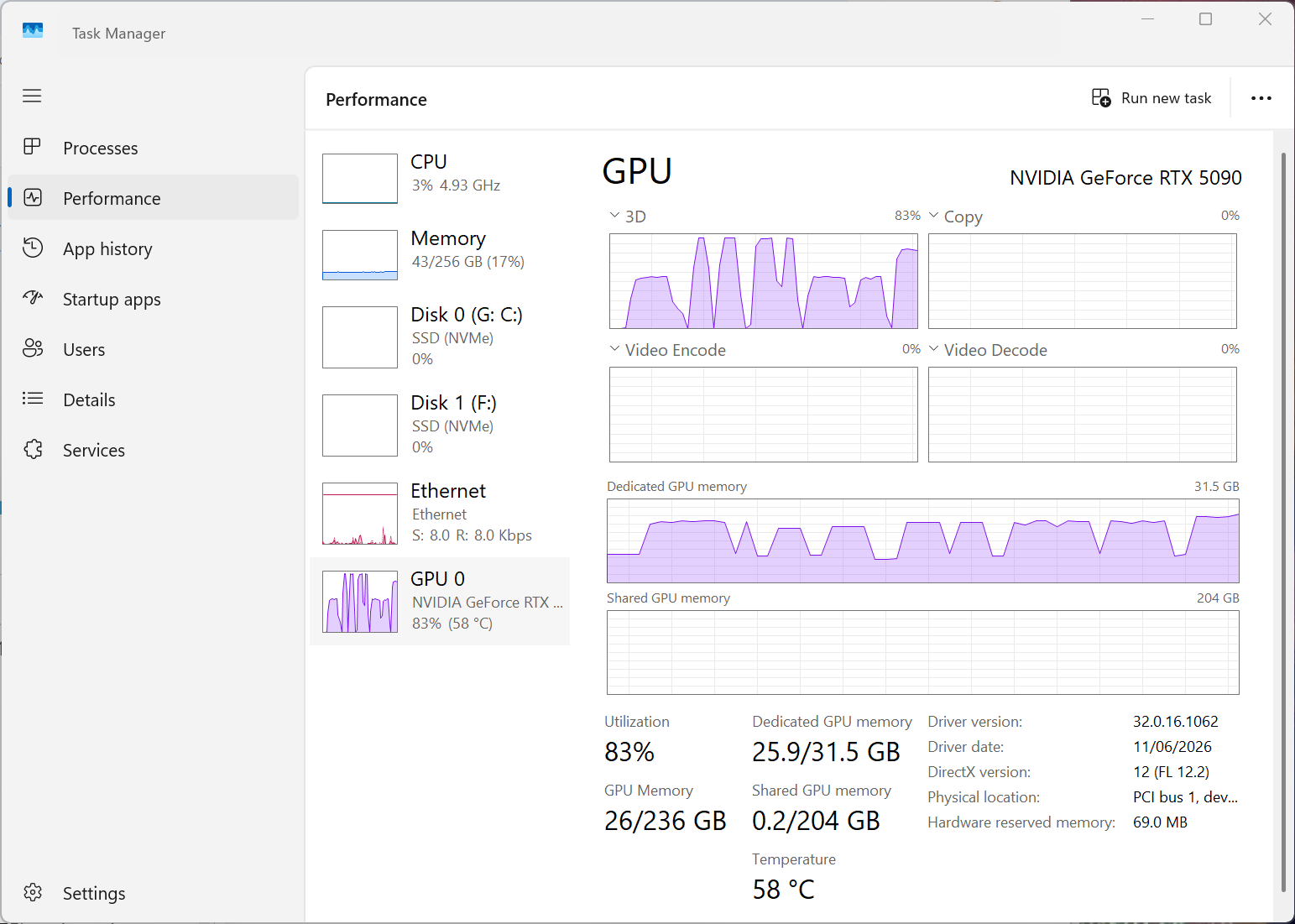
I noticed that GPU utilization of this example was low (about 20%). I decided to exercise Gemini and we worked out the vectorization of a loop that sped things up 4x. Strangely, utilization only rose to 40% or so. Here’s the change:

These are the measurements of the VFI loop after GEqm (which I obviously skip for benchmarking purposes, using tau=0.0975):

Original code; Elapsed time is 397.473481 seconds.

Vectorized code: Elapsed time is 106.088885 seconds.

Vectorized singlefp code: Elapsed time is 94.404304 seconds.

It needs work, but it shows promise…

2 Likes

Wait, what did you vectorize?

I was thinking you were going to say you vectorized d3 (the decision variable that drives the semi-exogenous shock). This is a clear target, I am just not sure what the runtime impact is.

But instead you vectorized the divide-and-conquer loop.

I can see both how vectorizing the DC-loop can help for some model, or hurt for some models. Obviously it increases the GPU memory demands. Less obvious is the runtimes. The DC is trying to take advantage of not having to look at all aprime (only those within the bounds determined by the monotonicity). By doing all of them in parallel I assume it had to do the ‘worst case length of the aprime range’ (since you have to have the same matrix dimension for everything). In a model where all the ‘length of aprime range’ for each ii is similar, this can clearly cut runtimes. In a different model where they was a large variance in the ‘length of aprime range’ across the ii it is possible it would hurt runtimes. [Note: this ‘worst case length of the aprime range’ is already applied to everything else, like over the d and z dimensions, but you now also apply it across the ii which is effectively the vfoptions.level1n dimension.]

I feel like the biggest weakness of this approach is simply that it make DC look much more like just running ‘without DC’ which is often not possible due to the memory demands. I guess this could be thought of a ‘halfway between with DC and without DC’ in terms of the memory use.

Given this model has n_d=101 for the driving decision variable (and could be run with 201) the parallel over ‘d3’ seems like it might hold promise, although it does risk blowing out memory use.

Still, cool to see that this ‘half DC’ approach is another possibility that the GPU seems to like, gives a small memory cut versus ‘no DC’, but can give meaningful speed improvement versus ‘full DC’.

Anyway, cool stuff :smiley:

PS. I wonder if a chunk of the gains you got could be had by playing with vfoptions.level1n?

When I looked at vectorizing d3, I saw too many moving parts for a first attempt. This smaller loop looked inviting. But now that you mention it, perhaps the easier approach would be to try some different options :wink:

What motivated me to give it a crack is that a few days ago I say performance drop off a cliff, and it was due to putting a gather statement inside a loop. When I saw very low GPU utilization it was a clue that something could be optimized.

Turning off divide and conquer drops the double precision runtime down to 79 seconds and the singlefp runtime down to 67 seconds. Memory utilization differences are negligible (reported 11.5 GB GPU RAM with or without DC).

This looks very promising, thanks for sharing! It applies to VF iteration with finite horizon, experience asset, grid interp layer and divide and conquer. I suspect however that the vectorization can be done to all finite horizon and grid interp layer commands (i.e. it is not specific to experience assets nor divide and conquer).

My takeaway is that I naively vectorized out what DC was trying to do, and that it is actually more efficient to just turn off DC in this particular case.

I’ve noticed in several other instances that turning on low memory options can actually speed things up rather than slowing them down, possibly because sending a large setup then doing a small calculation doesn’t pipeline as well as looping over smaller chunks whose small calculation do pipeline well.

Performance engineering is a bit of an art, and watching the GPU dashboard (and the clock) helps tell you when your model is in the weeds. How to find you way back to the course? We need a VFI for the VFIToolkit runtime options! :upside_down_face:

Now it gets interesting. I got some quick help vectorizing over d3 (which I had previously discussed as an idea with Robert), and here are the results:

Single FP (fits easily in 24 GB VRAM): Elapsed time is 60.143706 seconds.

Double FP (requires 45GB VRAM): Elapsed time is 237.005294 seconds.

Looped Single FP: Elapsed time is 76.044933 seconds.

Looped Double FP (requires only 9GB VRAM): Elapsed time is 78.137489 seconds.

Since my GPU has only 32GB VRAM, there’s a large performance hit as the card accesses “Shared GPU Memory”. SingleFP matrices save a lot of space in the VFI computation realm when VRAM is in high demand.

Is it worth vectorizing everything? Is it worth having a singlefp option? It all depends…

For the curious, here’s the vectorized loop (with commentary by Gemini):

% 1. Combine grids for N_d2 and N_d3
N_d23 = N_d2 * N_d3;
d23_gridvals_val_all = [repmat(d2_gridvals, N_d3, 1), repelem(d3_grid(:), N_d2, 1)];

% 2. Vectorize the Expected Value (EV) block over N_d3
pi_bothz_all = pi_semiz_J(:, :, :, jj); % Shape: [N_shocks, N_bothz, N_d3]
pi_bothz_perm = permute(pi_bothz_all, [2, 1, 3]); 
pi_bothz_shifted = reshape(pi_bothz_perm, [1, size(pi_bothz_perm, 1), size(pi_bothz_perm, 2), N_d3]);

EV_all = EVpre .* pi_bothz_shifted;
EV_all(isnan(EV_all)) = 0;
EV_all = sum(EV_all, 2);
EV_3D = reshape(EV_all, [N_a, N_bothz, N_d3]);

% 3. Extract lower and upper bounds using 4D expanded indices
% Push the N_d3 offset to the 4th dimension (1x1x1xN_d3) so it broadcasts properly
offset_d3 = reshape((0:N_d3-1) * (N_a * N_bothz), 1, 1, 1, N_d3);

% Now implicit expansion works: [201x51x4] + [1x1x1x101] -> [201x51x4x101]
lin_lower_3D = lin_lower + offset_d3;
lin_upper_3D = lin_upper + offset_d3;

EV1_3D = EV_3D(lin_lower_3D);
EV2_3D = EV_3D(lin_upper_3D);

skipinterp_3D = (EV1_3D == EV2_3D);

% Expand aprimeProbs_full along the 4th dimension to match
aprimeProbs_3D = repmat(aprimeProbs_full, 1, 1, 1, N_d3);
aprimeProbs_3D(skipinterp_3D) = 0;

entireEV_3D = EV1_3D .* aprimeProbs_3D + EV2_3D .* (1 - aprimeProbs_3D);

% 4. Compute DiscountedEV for the combined dimensions
DiscountedEV_3D = DiscountFactorParamsVec * reshape(entireEV_3D, [N_d2, N_a1, 1, N_a2, N_bothz, N_d3]);

% Merge d2 and d3 into the first dimension to run interp1 cleanly
DiscountedEV_merged = reshape(permute(DiscountedEV_3D, [1, 6, 2, 3, 4, 5]), [N_d23, N_a1, 1, N_a2, N_bothz]);
DiscountedEVinterp_merged = permute(interp1(a1_gridvals, permute(DiscountedEV_merged, [2,1,3,4,5]), a1prime_grid), [2,1,3,4,5]);

% 5. First CreateReturnFnMatrix call (Combined N_d23)
ReturnMatrix_all = CreateReturnFnMatrix_ExpAsset_Disc(ReturnFn, 0, [N_d23, 1], n_a1, n_a1, n_a2, n_bothz, ...
    d23_gridvals_val_all, a1_gridvals, a1_gridvals, a2_gridvals, bothz_gridvals_J(:,:,jj), ReturnFnParamsVec, 1, 0);

entireRHS_all = ReturnMatrix_all + DiscountedEV_merged;

% 6. First Max Operation and Midpoint calculations
[~, maxindex_all] = max(entireRHS_all, [], 2);

midpoint_all = max(min(maxindex_all, n_a1(1)-1), 2);
a1primeindexesfine_all = (midpoint_all + (midpoint_all - 1)*n2short) + (-n2short-1:1:1+n2short);

% 7. Second CreateReturnFnMatrix call (Refined Grid)
ReturnMatrix_ii_all = CreateReturnFnMatrix_ExpAsset_Disc(ReturnFn, 0, [N_d23, 1], n2long, n_a1, n_a2, n_bothz, ...
    d23_gridvals_val_all, a1prime_grid(a1primeindexesfine_all), a1_gridvals, a2_gridvals, bothz_gridvals_J(:,:,jj), ReturnFnParamsVec, 2, 0);

d2a1primea2bothz_all = (1:1:N_d23)' + N_d23*(a1primeindexesfine_all-1) + N_d23*N_a1prime*a2ind + N_d23*N_a1prime*N_a2*bothzind;
entireRHS_ii_all = ReturnMatrix_ii_all + reshape(DiscountedEVinterp_merged(d2a1primea2bothz_all(:)), [N_d23*n2long, N_a1*N_a2, N_bothz]);

% 8. Second Max Operation: Separate d2 and d3 to ensure max is ONLY taken over n2long and d2
% Reshape and permute so d3 is pushed to the back, allowing dim 1 max to work accurately
temp = reshape(entireRHS_ii_all, [N_d2, N_d3, n2long, N_a1*N_a2, N_bothz]);
temp = permute(temp, [1, 3, 4, 5, 2]); % -> [N_d2, n2long, N_a1*N_a2, N_bothz, N_d3]
temp = reshape(temp, [N_d2*n2long, N_a1*N_a2, N_bothz, N_d3]);

[Vtempii_all, maxindexL2_all] = max(temp, [], 1);
V_ford3_jj = shiftdim(Vtempii_all, 1); % Native [N_a1*N_a2, N_bothz, N_d3] shape

% 9. Linear Indexing updates and Policy creation
d_ind = rem(maxindexL2_all - 1, N_d2) + 1;
d3_offset_n2long = reshape(0:N_d3-1, 1, 1, 1, N_d3) * N_d2;
allind_all = (d_ind + d3_offset_n2long) + N_d23*aind + N_d23*N_a*bothzBind;

% No need to loop over d3_c, we assign the expanded dimensions directly
Policy3_ford3_jj(1, :, :, :) = d_ind;
Policy3_ford3_jj(2, :, :, :) = midpoint_all(allind_all);
Policy3_ford3_jj(3, :, :, :) = ceil(maxindexL2_all / N_d2);

% 10. Boundary flags setup
base_ind = d_ind + d3_offset_n2long;
jump_aind = (N_d23 * n2long) * aind;
jump_bothz = (N_d23 * n2long) * N_a * bothzBind;

linidx_lower_all = base_ind + jump_aind + jump_bothz;
linidx_upper_all = base_ind + N_d23*(n2long-1) + jump_aind + jump_bothz;

isInfLower_all = (ReturnMatrix_ii_all(linidx_lower_all) == -Inf);
isInfUpper_all = (ReturnMatrix_ii_all(linidx_upper_all) == -Inf);

L2offset_all = ceil(maxindexL2_all / N_d2);
inLowerStrict_all = (L2offset_all >= 2) & (L2offset_all <= n2short+1);
inUpperStrict_all = (L2offset_all >= n2short+3) & (L2offset_all <= n2long-1);

flag_ford3_jj = shiftdim(2 + (inLowerStrict_all & isInfLower_all) - (inUpperStrict_all & isInfUpper_all), 1);

One small note: I noticed that the initializations of lin_lower and lin_upper are loop-invariant, and so can be lifted out of all loops to where we initialize aprimeIndex_full and aprimeplus1Index_full even if we do not vectorize. I leave it to Claude Code to push that change everywhere.

And now a puzzler:

If I change the ExpAsset from 51 gridpoints to 31 (with an optimizer I’m testing to make it “just as good”) the GPU utilization jumps 2x (to 96%) and the overall GEqm is found in 1/3rd the time, even though 51/31 is suggests it should only be a 60% faster solve.

Using 21 gridpoints max utilization peaks at 94% (15/32 GB GPU).

Using 31 gridpoints max utilization peaks at 96% (21/32 GB GPU).

Using 41 gridpoints max utilization drops to 84% (26/32 GB GPU).

Using 51 gridpoints it’s stuck at 40% (30/32 GB GPU).

The 21-gridpoint solution misses the full-scale target by 0.0001 (0.0976 vs 0.0975) and reaches an asset level that’s short by 0.02 (i.e disagreement in the 3rd sig fig). Total calculation time: 05:57.

For run I attempted to map the origins of the chokepoint and found non-linear behavior. At 36 gridpoints there’s a big drop down to 55%. In this screenshot you can see the peaks at 33 and 34, the big drop at 36, and the climb back up to 84% at 41.

I agree. I think that the parallel over ii was close to turning off divide and conquer (not quite the same, but close to it). That said, was cool to see that can turn off divide-and-conquer in this model (I am going to try it on my desktop later). Kind of makes sense after seeing it, because it is looping over d3, so there is just the one standard endogenous state, plus the experienceassetsemiz but that is only this period value, and the semi itself is just four values. But I wouldn’t have thought it would fit in memory without seeing it first.

Hmm, the one time I did parallel the decision variable controlling the semi-exogenous state the runtime gains were a lot smaller than I had hoped. I think the key will be in exactly how the parallelization proceeds and the interaction with semi-exo transition probabilities, will need to be done just right to see real gains.

1 Like

So I asked the Googles this question: “what sizes and shapes of matrices cause arrayfun to increase/decrease gpu utilization for 5-d matrices that easily fits in vram?”

And got a pretty useful answer that chimes with what I reported (small changes to shapes can affect performance 2x):

At the end is the body text referenced in the above search link.

It strikes me that (1) the toolkit could easily provide some warnings about grid shapes that are problematic. And (2) Given that in more than a few cases we see smaller-dimensioned decision variables in front of larger-dimensioned endogenous variables, it might be beneficial to have a translation layer between the ReturnFn (or aprimeFn) that we declare and the ReturnFn we call.

Regarding (2), I think it’s a great feature that the toolkit provides a highly regular order of variables so that people can feel comfortable and confident as they develop their models and the functions that operate on them. But if we insert some shim functions, we can declare everything the way the toolkit is documented, but organize the data we pass to arrayfun and and reorganize the way our ReturnFn (or aprimeFn) is called so that we see everything in the order we expect, even though we reordered it so that the GPU can really scream.

The utilization factors that sent me on this vectorization journey show that there are substantial peroformance gains that can be achieved by organizing things so that each of the 32 vector units is cranking away in parallel in a good way, and not each hammering the same block at the same time, resulting in a complete serialization of the program. The explanation below clearly shows that a “spray and pray” approach to putting everything in memory is less optimal than putting it carefully into memory. And this explains why I have seen some cases where looping through a particular variable (via lowmemory==1 or lowmemory==2) can be preferable to lowmemory==0.

Google’s answer:

Shapes that Increase GPU Utilization (High Efficiency)

To maximize your Streaming Multiprocessor (SM) occupancy and memory bandwidth, your 5-D matrix should favor the following configurations:

  • Large Total Element Count (\(> 1,000,000\) elements): The 5-D matrix must be large enough to spawn tens of thousands of threads. If the total product of the dimensions (\(N_1 \times N_2 \times N_3 \times N_4 \times N_5\)) is too low, there will not be enough parallel threads to hide the memory latency. [1]

  • Large First Dimension (Stride-1 Layout): MATLAB uses column-major order. The GPU threads map sequentially to the first dimension. Ensuring that Dimension 1 is large (e.g., \(512 \times 32 \times 32 \times 4 \times 4\)) allows multiple threads in a CUDA warp to read contiguous memory addresses simultaneously (coalesced memory access). [1, 2, 3]

  • Dimensions Modulo 32 (Warp Alignment): Matrix shapes where the inner dimensions are multiples of 32 (e.g., \(64 \times 32 \times 32 \times 32 \times 32\)) align perfectly with the GPU’s 32-thread warps. This eliminates tail-end threads that waste execution cycles. [1]

Shapes that Decrease GPU Utilization (Low Efficiency)

Even if a 5-D matrix comfortably fits in VRAM, certain shapes will force the GPU to stall, causing compute utilization to drop to single digits:

  • Tiny First Dimension (“Flat” Column Vectors in N-D Space): A shape like \(1 \times 100 \times 100 \times 100 \times 10\) is devastating for arrayfun. Because data is read sequentially across rows/pages instead of down columns, adjacent GPU threads must access memory locations that are wildly spread apart. This breaks coalescing and forces the memory controller to perform serial transactions. [1, 2, 3, 4, 5]

  • Highly Mismatched Sizes utilizing Implicit Expansion: If you are passing multiple 5-D matrices into arrayfun (e.g., Matrix A is \(100 \times 1 \times 100 \times 1 \times 50\) and Matrix B is \(1 \times 100 \times 1 \times 100 \times 50\)), MATLAB will implicitly expand them. While convenient, the complex underlying index arithmetic required to calculate source memory locations for each thread overpowers the actual math operation, creating massive instruction overhead. [1]

  • Small Total Matrix Sizes: A 5-D matrix like \(4 \times 4 \times 4 \times 4 \times 4\) has only 1,024 elements. This will completely starve a modern GPU, resulting in near 0% volatile GPU utilization because the kernel initialization overhead takes longer than the actual execution. [1, 2]


Quick Optimization Matrix

5-D Matrix Shape Example Total Elements Performance Impact Primary Reason
512 x 64 x 32 x 16 x 8 ~268 Million Excellent :rocket: Large Dim 1, warp-aligned, hides latency.
undefined ---- ---- ----
1,000,000 x 1 x 1 x 1 x 1 1 Million Good :+1: Acts as a long 1D vector; excellent memory coalescing.
undefined ---- ---- ----
1 x 1 x 32 x 32 x 32 32,768 Poor :chart_decreasing: Total element count is too low to fill GPU cores.
undefined ---- ---- ----
2 x 512 x 512 x 4 x 4 ~8.3 Million Terrible :cross_mark: Dim 1 breaks memory coalescing; causes unaligned reads.
undefined ---- ---- ----

Summary Recommendation

If you have control over how your 5-D data is structured, always push your largest and most continuous tracking dimension to the front (Dimension 1). If your matrix must have small singleton dimensions, try to keep them at the tail end (Dimensions 4 and 5).

If you are profiling your code, make sure to wrap your tests in gputimeit rather than tic/toc to ensure you are measuring true GPU kernel execution time instead of CPU-GPU host synchronization lag. [1]

1 Like

The Quick Optimization Matrix is very useful, thanks! Important message: make sure the first dimension is large enough, because of Matlab column-major ordering.