Fast Distribution (based on E. Tan, Econ Letters 2020)

[aledinola]

There is a very interesting paper by Eugene Tan (University of Toronto), “A Fast and Low Computational Memory Algorithm For Non-Stochastic Simulations in Heterogeneous Agent Models”, published in Economic Letters, link here

The paper provides a new method to compute the stationary distribution in heterog agents economies, which is faster and less memory-demanding than the textbook method (as described e.g. in Liunqvist and Sargent textbook).

In a nutshell, the standard method relies on computing a big transition matrix that gives the probability of moving from point (a,z) today to point (a’,z’) tomorrow, where a denotes the endog state and z is the exog state (I follow the standard notation of the toolkit). Unfortunately this object is often large (even if it is built as a sparse matrix) and can become not manageble if the state space is too big.

Eugene’s method instead split the problem in two parts: first, compute the transition operator from (a,z) to (a’,z), fixing z at today’s level. Then do a matrix multiplication to update z using the exogenous transition matrix pi_z. The paper provides a great explanation and offers much more detail than I can do here of course.

I have implemented Eugene’s method in Matlab within the toolkit. I modified a few lines of the toolkit function StationaryDist_Case1.m (see code below). Then I added the function StationaryDist_Case1_Iteration_raw_AD. If the user selects

simoptions.method = ‘AD’

then the toolkit will call the new function StationaryDist_Case1_Iteration_raw_AD and solve the distribution using the new method. If instead the user writes

simoptions.method = ‘RK’

the toolkit will call the function StationaryDist_Case1_Iteration_raw and use the standard method.

It is important to initialize simoptions.method to either ‘AD’ or ‘RK’, otherwise the code will throw an error.

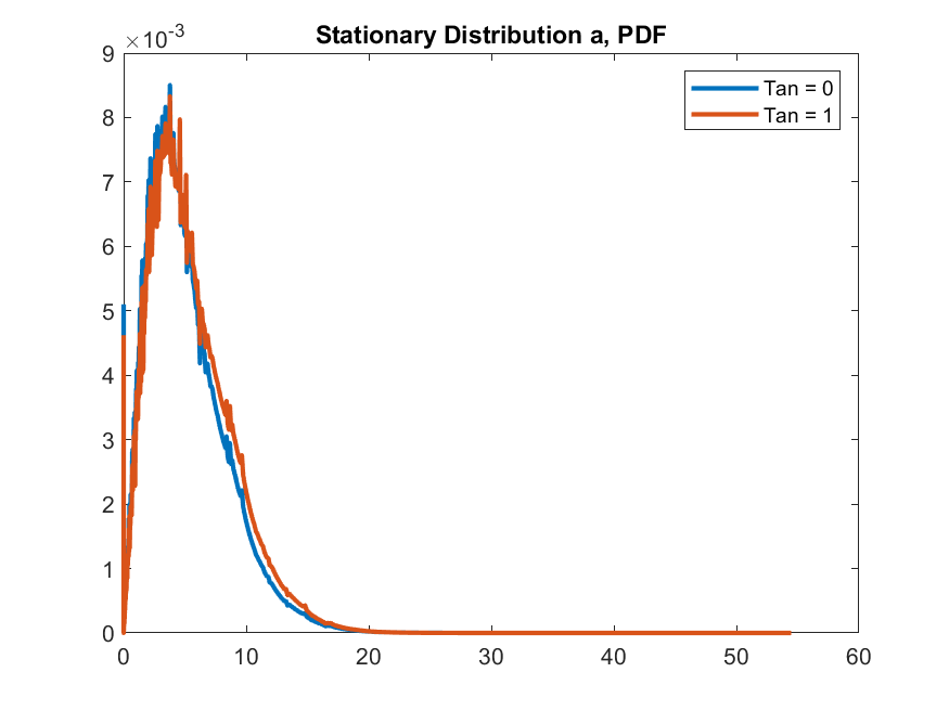
I provide an example using Aiyagari’s model on my github page

GitHub - aledinola/FastDistribution: Implementation of Eugene Tan's method to...

I rely on Robert’s Aiyagari example and show that the new method is about 12 times faster than the standard method, given a parametrization with n_a=512 and n_z=21, everything else as in Robert’s example.
A disclaimer: my code is tested only for the simplest case with infinite horizon, no d variable, no semi-endogenous shocks, etc. (so, basically, Aiyagari 1994).

Let me know what you think!

Here is the modification to the toolkit function StationaryDist_Case1.m

%% Iterate on the agent distribution, starts from the simulated agent distribution (or the initialdist)
if simoptions.iterate==1
if strcmp(simoptions.method,‘RK’)
StationaryDistKron=StationaryDist_Case1_Iteration_raw(StationaryDistKron,PolicyKron,N_d,N_a,N_z,pi_z,simoptions);
elseif strcmp(simoptions.method,‘AD’)
StationaryDistKron=StationaryDist_Case1_Iteration_raw_AD_vec(StationaryDistKron,PolicyKron,n_d,n_a,n_z,pi_z,simoptions);
end
end

[robertdkirkby]

This is sweet! I am going to call this the “Tan improvement”

I have implemented Tan improvement for iterating the agent distribution in infinite horizon, and made it the default. I also made refinement the default for the value fn. Between the two it should cut runtimes for Aiyagari (1994), and especially for the extension to endogenous labor (so Pijoan-Mas, 2006).

The speed gain is roughly cutting the runtime for agent stationary distribution by about one order of magnitude; considering only the part of the code that does the iteration itself. Because iteration is only part of it (there is some simulation to get an initial guess) the total runtime for the agent stationary distribution is about one-third what it was. [Also, your codes use tolerance for value fn convergence as max(abs()) while toolkit uses sum(abs()) so your codes are a bit faster still for this reason.]

Given how fast iteration now is, I suspect the toolkit is doing too much simulation to generate the initial guess for the agent distribution, and speeds could be improved by cutting this back a bit.

I still need to look more at how the speed gains interact with sparse/full matrices, and with gpu. I suspect there are further speed gains to be had by choosing the right combo for the Tan improvement.

I also expect the Tan improvement is going to lead to even larger speed gains in finite horizon, as there computing the full transition matrix for (a,z) [what VFI Toolkit calls P, and Tan (2020) calls That] takes most of the runtime and Tan improvement means we don’t need to compute it at all.

Hopefully I can roll it out more widely over the next week or two. Is going to be a fair bit of work, but given the clear speed improvement, and even loosening memory bottlenecks, it should be well worthwhile.

Internally I have set the default to be simoptions.tanimprovement=1, which uses the Tan improvement when performing iteration.

And thanks for setting up the example code! I think it would have taken me a good two or three days from scratch, but with your example code to work with I was able to figure it out in one morning as I could easily see which of my steps were working and which were not.

[Comment: Tan (2020) has the distribution as (z,a), in VFI Toolkit it is (a,z). He explains the two steps of the “Tan improvement” in his Section 2.2. Hence his first step is Gamma x Lambdahat, and it is the same in toolkit except that both Gamma and Lambdahat are based on (a,z) rather than his (z,a). His second step is pi_z’ x Lambdatilde, and in toolkit this is just pi_z*Lambdatilde (h is his notation for pi_z).]

[robertdkirkby]

Hmm, one complication is that while matlab does have sparse gpu arrays, you cannot use reshape() on them.

I did some speed comparisons and Tan improvement on sparse cpu arrays seems to be faster than traditional iteration with gpu arrays (sparse or full), so I guess I will just make is so that default will always be to move everything to cpu and do Tan improvement there.

That you can switch from gpu to cpu for a bunch of matrix operations and still be one-third the run time shows just how good the Tan improvement is here.

If anyone can see how to do Tan improvement without the need to reshape() please let me know as could then implement it with sparse gpu arrays, presumably would be faster still.

[robertdkirkby]

Ran a test on just using a very naive initial guess for distribution. It was substantially faster thanks to Tan improvement. I have now pushed this too.

Runtime for agent distribution in Aiyagari (1994) example is now about one-tenth what it was.

Next is just to roll this out everywhere

[aledinola]

Hi Rob,

great that you have already implemented the Tan improvement in the VFI toolkit codes! I have tested the Aiyagari example again on the new codes (downloaded from github) and I have a couple of observations:

1. When I run aiyagari I get a warning since refinement is ON but there is no d variable. I think if there is no d variable the default should be

vfoptions.solnmethod = ‘purediscretization’; % since there is no d variable

2. I ran the distribution twice, with the Tan improvement to 0 and to 1, respectively. With the default tolerance (1e-6 in the L1 norm) there are some (small?) discrepancies between the two methods (see plot). I found this a bit suspicious since mathematically the two methods are equivalent… but maybe some rounding error? [I got the same issue in my codes, so it does not depend on the way we coded it up]

From the plot you can see that the discrepancy is clearly visible.
Good news is that if I set

simoptions.tolerance = 1e-8

that the two graph not different anymore. Still a small numerical difference though…

I copy down here my codes

%simoptions.tolerance = 1e-8; %Deafult is 10^(-6)

simoptions.tanimprovement = 0;

tic

StationaryDist_0=StationaryDist_Case1(Policy,n_d,n_a,n_z,pi_z, simoptions);

time_0 = toc;

fprintf('Tanimprovement = 0: Time to solve for distribution: %f \n',time_0)

simoptions.tanimprovement = 1;

tic

StationaryDist_1=StationaryDist_Case1(Policy,n_d,n_a,n_z,pi_z, simoptions);

time_1 = toc;

fprintf('Tanimprovement = 1. Time to solve for distribution: %f \n',time_1)

fprintf('Speed-up of Tan improvement vs default: %f \n',time_0/time_1)

err_0_1 = max(abs(StationaryDist_0(:)-StationaryDist_1(:)));

fprintf('Discrepancy between two method: %f \n', err_0_1)

StationaryDist_0_a = get_marginal(StationaryDist_0);

StationaryDist_1_a = get_marginal(StationaryDist_1);

Policy = squeeze(gather(Policy));

PolicyVal = a_grid(Policy);

figure

plot(a_grid,a_grid,'--','LineWidth',2)

hold on

plot(a_grid,PolicyVal(:,1),'LineWidth',2)

hold on

plot(a_grid,PolicyVal(:,end),'LineWidth',2)

legend('45 line','low z','high z')

title('Policy function assets a')

figure

plot(a_grid,StationaryDist_0_a,'LineWidth',2)

hold on

plot(a_grid,StationaryDist_1_a,'LineWidth',2)

legend('Tan = 0','Tan = 1')

title('Stationary Distribution a, PDF')

print('pdf_assets','-dpng')

[robertdkirkby]

Cleaned it up so that default is to use refinement, but if it notices you have no d variable then it turns off refinement as it would not actually do anything.

Note that part of the reason your earlier code gave slightly different answer was that you have tolerance criteria measuring distance as max(abs()), while VFI Toolkit uses sum(abs()).

Your (2) will be about numerical rounding errors being different with and without Tan improvement. I guess maybe I should run some speed tests to see if Tan improvement with tighter tolerance criterion makes sense.

I ran the full code for Aiyagari (1994) model, the run times are notably faster (less than half). I then did the version with endogenous labor (Pijoan-Mas 2006 model) and running with both refinement and Tan improvement versus what it used to be without them the speed gains are measured in orders of magnitude. Seriously nice.

[Further speed gains could be easily had if you were to use shooting algorithm for the general eqm conditions rather than the default; appendix to the Intro to OLG Models explains how to set this up.]

[robertdkirkby]

While I am thinking about agent distributions I added computing the stationary distribution in infinite horizon models to the Pseudocodes, should help make clearer what all the options are.

[aledinola]

I’m really happy that the Tan improvement makes the codes so much faster!

A wild thought: could the Tan improvement also help with the Howard? The idea would be to code the Howard improvement using sparse matrices (not loops as it is done now in the toolkit, which does about 80 Howard iterations) as it explained in Sargent’s textbook (see chapter on Practical dynamic programming) and recently done in a paper by Pontus Rendhal. Then the matrix Gamma (see Robert’s pseudocode) can be used for both the Howard and for the distribution (killing two birds with one stone)

When coding myself the Howard improvement I typically do it as in the toolkit because the matrix-based approach is often too memory-demanding. But with the Tan improvement it is much less so.

Sorry if all this seems not very clear, if I have time I’ll try to think more about it and re-write this post in a clearer language

[robertdkirkby]

Any meaningful speed improvements you want to demonstrate for toolkit commands, I am happy to roll them out

Right now though you’ve already given me about a week’s work rolling out this Tan improvement everywhere, that is enough for me for the moment

[robertdkirkby]

Rolled out Tan improvement to most of the toolkit, should be done by end of the week.

Gains in finite horizon are solid, but not a full order of magnitude like for infinite horizon. Definitely worth implementing and I made some other small improvements while I was there. Other difference is that there are lots of models where you couldn’t do traditional iteration but Tan improvement iteration will work as it is less demanding of memory.

One place I cannot implement it (unless I missed something) is semi-exogenous shocks, which gives some good intuition into why the Tan improvement boosts speed: In standard setup we have Policy from (a,z) to a’, and pi_z from z to z’. Tan improvement is to start from (a,z), use Policy to go to (a’,z), then use pi_z to get (a’,z’). Traditional iteration builds P from (a,z) to (a’,z’). Tan improvement is faster because it takes advantage of the fact that z’ does not depend on a. When we construct P we are considering the possibility of (a,z) to z’, which wastes a lot of computation because z’ does not depend on a. This to my mind is the key to Tan improvement, you don’t waste time dealing with the potential for z’ to depend on a (as well as z); we know it doesn’t, so don’t compute as if it might. [Saying the same a different way: We start from (a,z). Tan step 1 uses this to get a’, we can then throw away a and just use z to get z’ in Step 2. This works and boosts speed because z’ does not depend on a. Whereas creating P makes z’ depend unnecessarily on a.]

This also illustrates why Tan improvement can’t be used for semi-exogenous shocks. Semi-exogenous shocks have transition probabilities that depend on (d,z). So their transitions are (d,z) to z’. Because policy for d is a function of (a,z) we can think of the semi-exogenous shocks as being from (a,z) to z’ [substitute d with (a,z)]. Hence there is nothing to be gained by the Tan improvement as the z’ do depend on a.

[robertdkirkby]

24 days later, so much for end of the week. Finally finished rolling out the Tan improvement. Phew! [Not all pushed yet, but will be in near future. Improvements are everywhere, especially nice with fastOLG mode in OLG transition paths.]

A quick comment on using Tan improvement in portfolio choice models (or any model where an iid shock occurs between this period decisions and next period endogenous state; what VFI Toolkit calls a u shock). Notice that when you have a u shock you will sometimes get the same grid index for lower grid point from one value of u and upper grid point of another value of u [upper and lower refer to interpolating back onto the grid]. Turns out Matlab’s sparse() command automatically sums the two values when an index is repeated, which is anyway exactly what you want to do to create Gamma for step 1 of the Tan improvement. Got lucky

[robertdkirkby]

Turns out I was not finished rolling out the Tan improvement.

Have just implemented Tan improvement for models with semi-exogenous shocks. While you cannot apply the Tan improvement to the semi-exogenous shocks themselves, if the model also includes exogenous shocks then you can apply the Tan improvement to these.

A brief explanation: start with standard Tan improvement, we want to go from current agent distribution on (a,z) to next period agent dist on (a’,z’). Before Tan, the standard approach is to use the policy, g, and exogenous shock transition matrix/kernel, pi_z, together to create T which is a markov transition matrix/kernel from (a,z) to (a’,z’). Tan improvement is to do conceptually the same in a computationally more efficient way. First step, create G from g, which goes from (a,z) to (a’,z), and then multiply this by the original distribution. Second step, just use pi_z to go from (a’,z) to (a’,z’).

When we have semi-exogenous shocks we want to get from the current agent distribution on (a,semiz,z) to the next period agent dist on (a’,semiz’,z’). Before Tan, the standard approach is to use the policy, g, and exogenous shock transition matrix/kernel, pi_z, and the semi-exogenous transitions, pi_semiz (which depends on g), together to create T which is a markov transition matrix/kernel from (a,semiz,z) to (a’,semiz’,z’). Tan improvement is to do conceptually the same in a computationally more efficient way. First step, create G from g and pi_semiz, which goes from (a,semiz,z) to (a’,semiz’,z), and then multiply this by the original distribution. Second step, just use pi_z to go from (a’,semiz’,z) to (a’,semiz’,z’). Because semiz is typically only a few grid points (employed/unemployed, or a handful of children), G is still very sparse and so we get a big speed boost (as well as cutting a memory bottleneck).

Note that implementing this Tan improvement for semi-exogenous shocks efficiently requires the ordering (a,semiz,z). Hence I have also had to make a breaking change to adopt this ordering (previously the toolkit was using (a,z,semiz)).

[robertdkirkby]

Just implemented Tan improvement to models with firm entry/exit. Typically this involved encoding exit into Gammatranspose, using pi_z as standard, and then adding a third step to handle the firm entry.

I think that is it for the Tan improvement, it now does everything in the toolkit involving agent distribution iteration.

[Speed gains were minimal, but mostly just because those firm entry/exit model examples were already so fast as the models are small, the agent distributions are now something like 0.03 seconds instead of 0.04 seconds without Tan improvement]