Hi, everybody:
I have a question about the no- borrowing budget constraint.
Let us see a simple case:
V(a_t) = max{u(c_t)+V(a_{t+1})}
subject to
(1) c_t + a_{t+1}= (1+r)*a_t
(2) a_{t+1}>=0
where u(c_t) is the utility function, c_t is consumption, r is a constant interest rate and a_t is asset holding.
Or we can use {a,c,aprime} to describe it again:
V(a) = max{u(c)+V(aprime)}
subject to
(1) c+ aprime= (1+r)*a
(2) aprime>=0
So, my question is how does the budget constraint (2) aprime>=0 apply to VFI, and how does VFI ensure that the calculation results meet the budget constraint (2)?
Thank you!
1 Like
Hi Tony,
there are two possible ways to enforce the budget constraint. In most of the example codes it is simply done via the grid on assets (the same grid applies to assets and next period assets). For example, we could set asset grid,
n_a=501; % Number of points to use for asset grid
a_grid=linspace(0,15,n_a)';
Because this grid has a minimum of zero, we are implicitly enforcing that a_{t+1}>=0.
The other alternative would be to use the return function. Say we have the grid
a_grid=linspace(-3,15,n_a)';
we could add the following lines to the return function
if aprime<0
  F=-Inf;
end
Because the return to choosing aprime<0 is minus infinity we would never choose it, which is effectively the same thing as making it impossible to choose (mathematically it is the same).
Which of the two should you use? If you know the value of the borrowing constaint (zero in your example) before you start then hardcoding it into the grid is the best approach. Notice that the second approach ‘wastes’ all the points on the asset grid that are below zero. Sometimes though you want to vary the borrowing constraint, for example maybe people without houses cannot borrow but people with houses can borrow (using the house as collateral), in which case the second approach of using the return function to enforce the constraint is likely better.
PS. The asset grid above is not very good because it has evenly spaced points. We know (from theory and experience) that the value function will have more curvature near the borrowing constraint. And for a given number of grid points we will get more accurate results if we put more points where there is most curvature (intuitively, high curvature means the first derivative is changing a lot, and so the choices, which are determined at the margin/by equating derivatives, are sensitive to changes in this region). So a better grid would be
a_grid=15*(linspace(0,1,n_a).^3)';
(this is also from 0 to 15, the power of three means more will be near 0; a higher power would distribute them even more towards zero; note that you could add/subtract if you want the minimum grid point to be something other than zero)
PPS. All grids must be column vectors. Hence the ’ on the linspace.
PPPS. Obviously all of these grids are enforcing a maximum of 15. As long as this number is ‘large enough’ it doesn’t matter. How big exactly ‘large enough’ is will depend on the model.
1 Like
Dear Robert:
Thanks for your answer!
Best,
Tony
Continuing the discussion from How to deal with no-borrowing budget constraint?:
Continuing the discussion from How to deal with no-borrowing budget constraint?:
Dear Robert:
I am doing investigation on VFIToolkit and I meet a question here.
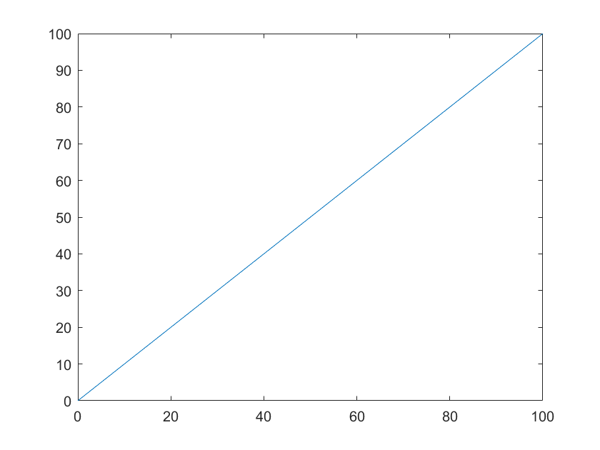
If I set the return function as a log-utility form,
F=log(c_t),
the policy function is linear.
But if I set the return function in the form of CRRA,
F= (c_t^(1-gamma)-1)/(1-gamma),
the outputted Policy seems not right, especially at the grid point a_grid=0, the consumption seems to be negative.
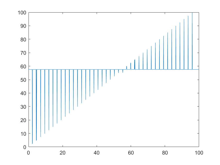
So why do this situation happen?
And how to deal with the CRRA in VFIToolkit?
Thank you!
Best,
Tony
1 Like
It seems that if I add if c>0 in the return function of the CRRA case, the plot is right.
Tony sent me codes by email and the issue was the following, which I repost here to help anyone who has similar issue. Tony actually figured it out in the meantime anyway 
Your code for the return function with log utility as the lines that relate to:
F=-Inf;
if c>0
    F=log(c);
end
whereas your codes for CRRA utility do not impose that utility is -infinity when c<0. They just say
F=(c^(1-gamma)-1)/(1-gamma);
and as a result there is no hard rule against choosing negative consumption.
The should impose it in the same manner, namely:
F=-Inf;
if c>0
    F=(c^(1-gamma)-1)/(1-gamma);
end
1 Like
Dear Robert:
Thanks for your reply again!
Best,
Tony