LifeCycleProfiles_FHorz_Case1_PType: Bug or Inconsistency for second-order and higher moments

aledinola · July 2, 2026, 2:53pm

In a previous post, Fortran vs VFI-Toolkit, I have highlighted that there is an inconsistency in the calculation of lifecycle moments with Ptypes for standard deviation, Gini coefficient etc. (basically eveything beyond the first moment).

My previous post was actually about a comparison between a Fortran implementation and the toolkit implementation of a lifecycle model, which found that the toolkit is competitive. This post instead focuses not on performance but on the apparent inconsistency mentioned above.

I have a very basic lifecycle model with exogenous labor supply (hence the only decision is savings) with state space given by

a assets
y Markov productivity shock
\theta permanent type
j age

I solve the model with the Toolkit in two ways:

Model 1: \theta is included as a second Markov shock, so z = [y;theta] and \theta has transition matrix with ones on the main diagonal and zeros elsewhere.
Model 2: \theta is handled as a permanent type, so z=y and \theta is a permanent type.

The test is to calculate average assets and the standard deviation of assets conditional on age j=1,...,N_j across the two methods. The two methods give identical results for the averages but different results for the standard deviations. The results generated by method 1 are the correct ones.

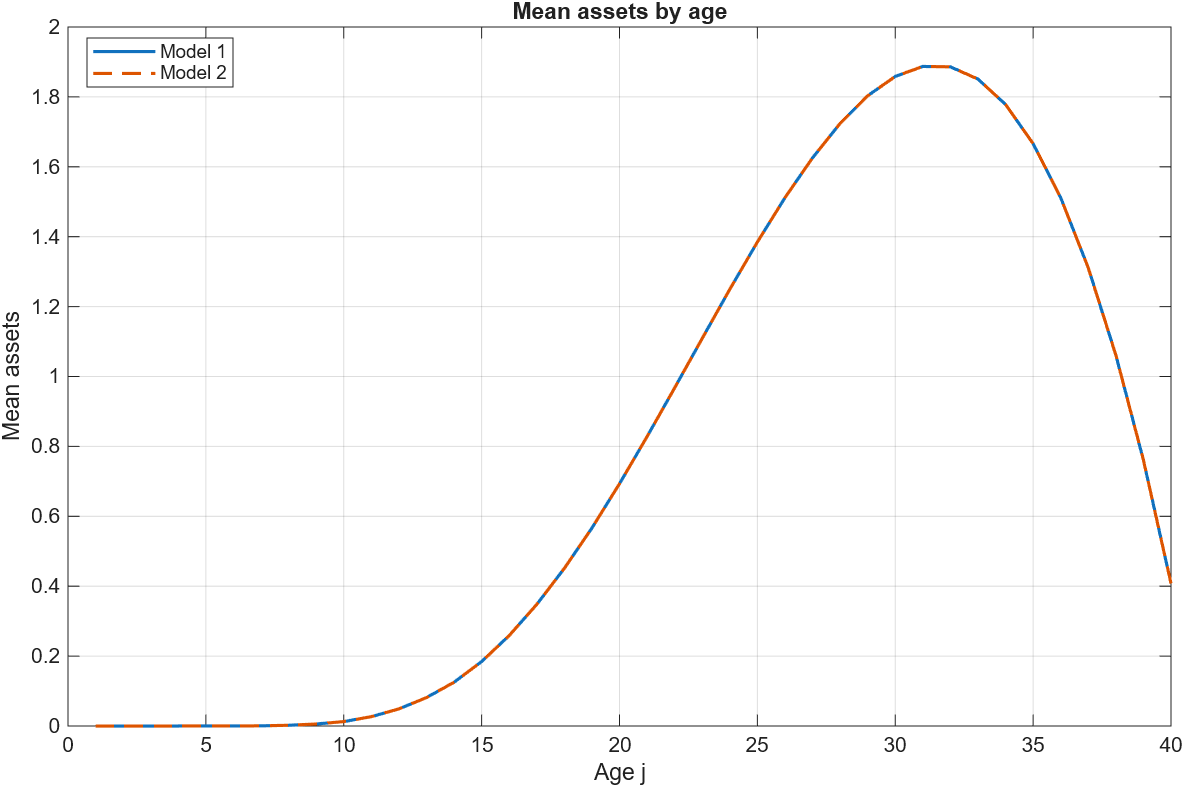
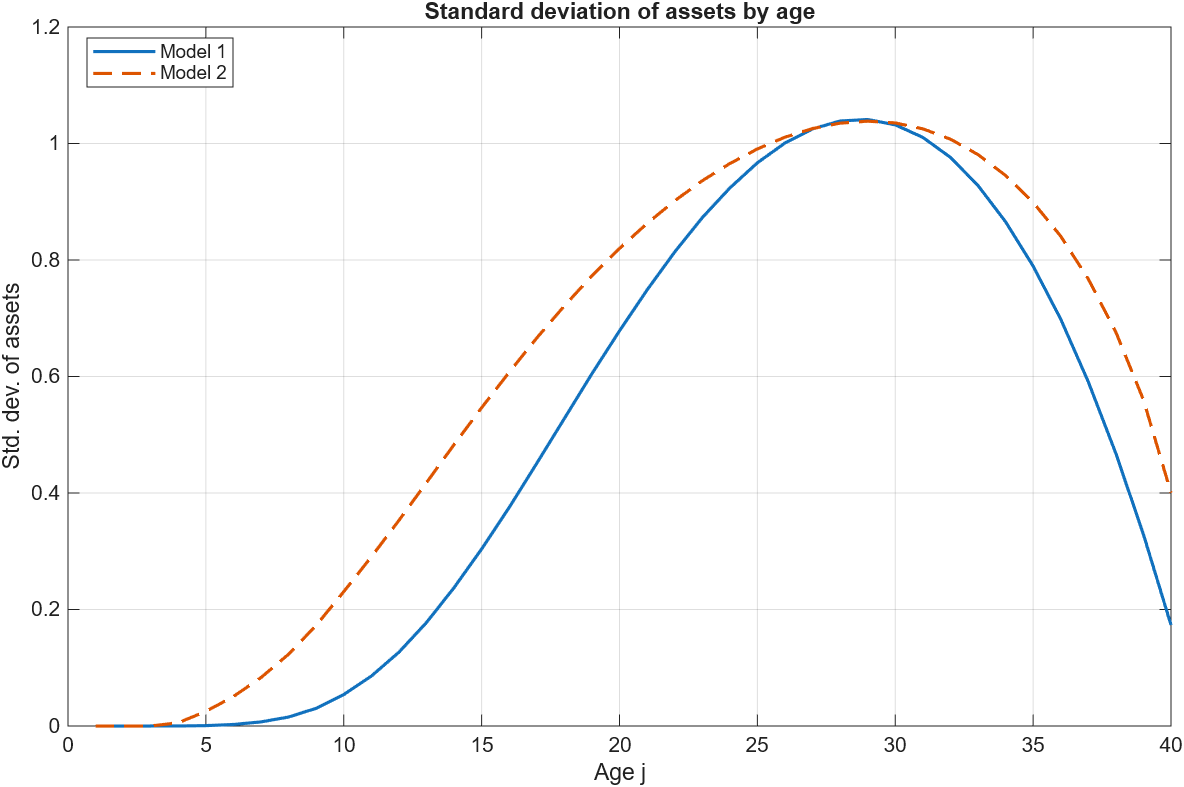
Here is the script:

%% basic_lifecycle_ptype_vs_markovshock.m
% Compare two equivalent ways to solve a lifecycle model in VFI Toolkit.
%
% Model 1: theta is included as a second Markov shock.
% Model 2: theta is handled as a permanent type.
%
% States:
%   a      assets
%   y      Markov productivity shock
%   theta  permanent type
%   j      age
%
% Choice:
%   aprime next-period assets

clear; clc; close all;
addpath(genpath('C:\Users\aledi\Documents\GitHub\VFIToolkit-matlab'))

%% Parameters

Params.beta  = 0.96;
Params.sigma = 2.0;
Params.r     = 0.03;
Params.w     = 1.0;

N_j = 40;
Params.N_j = N_j;

Params.ej = 0.7 + 0.6*sin(pi*(1:N_j)/N_j);

%% Grids

n_a = 201;
a_grid = 20*(linspace(0,1,n_a).^2)';

n_y = 7;
rho_y = 0.90;
sigma_y = 0.15;
sigma_eps_y = sqrt(1-rho_y^2)*sigma_y;
Tauchen_q = 3;

% Toolkit Tauchen routine.
[logy_grid, pi_y] = discretizeAR1_Tauchen( ...
    0, rho_y, sigma_eps_y, n_y, Tauchen_q);

% Convert log y to levels and normalize E[y]=1.
y_grid = exp(logy_grid(:));
[mean_y,~,~,~] = MarkovChainMoments(y_grid, pi_y);
y_grid = y_grid / mean_y;

% Initial y distribution: all mass on y_grid(4).
pi0_y = zeros(n_y,1);
pi0_y(4) = 1;

% Permanent types.
theta_grid = [0.75; 1.00; 1.25];
n_theta = numel(theta_grid);

pi_theta = eye(n_theta);

pi0_theta = [0.25; 0.50; 0.25];
pi0_theta = pi0_theta / sum(pi0_theta);

%% Toolkit setup

n_d = 0;
d_grid = [];

DiscountFactorParamNames = {'beta'};

Params.mewj = ones(1,N_j)/N_j;
AgeWeightParamNames = {'mewj'};

vfoptions = struct();
vfoptions.verbose = 1;

simoptions = struct();

%% ========================================================================
% Model 1: theta as second Markov shock
% ========================================================================

fprintf('\nSolving Model 1: theta folded into z=(y,theta)...\n');

Params1 = Params;

% z = (y,theta), with y varying first:
%   (y1,theta1), ..., (yN,theta1),
%   (y1,theta2), ..., (yN,theta2), ...
n_z1 = [n_y, n_theta];

z_grid1 = [y_grid; theta_grid];

% Since y varies first, use kron(pi_theta,pi_y).
pi_z1 = kron(pi_theta, pi_y);
pi0_z1 = kron(pi0_theta, pi0_y);

% Initial distribution over (a,y,theta) at j=1.
jequaloneDist1 = zeros(n_a,n_y,n_theta);
jequaloneDist1(1,:,:) = reshape(pi0_z1,[1,n_y,n_theta]);

ReturnFn1 = @(aprime,a,y,theta,sigma,r,w,ej) ...
    lifecycle_returnfn(aprime,a,y,theta,sigma,r,w,ej);

[V1, Policy1] = ValueFnIter_Case1_FHorz( ...
    n_d, n_a, n_z1, N_j, ...
    d_grid, a_grid, z_grid1, pi_z1, ...
    ReturnFn1, Params1, DiscountFactorParamNames, [], vfoptions);

StationaryDist1 = StationaryDist_FHorz_Case1( ...
    jequaloneDist1, AgeWeightParamNames, Policy1, ...
    n_d, n_a, n_z1, N_j, pi_z1, Params1, simoptions);

FnsToEvaluate1.assets = @(aprime,a,y,theta) a;
FnsToEvaluate1.income = @(aprime,a,y,theta,w,ej) w*theta*y*ej;

AgeConditionalStats1 = LifeCycleProfiles_FHorz_Case1( ...
    StationaryDist1, Policy1, FnsToEvaluate1, Params1, [], ...
    n_d, n_a, n_z1, N_j, d_grid, a_grid, z_grid1, simoptions);

fprintf('Model 1: size(V1) = [%s]\n', num2str(size(togather(V1))));

%% ========================================================================
% Model 2: theta as permanent type
% ========================================================================

fprintf('\nSolving Model 2: theta as permanent type...\n');

Params2 = Params;

n_z2 = n_y;
z_grid2 = y_grid;
pi_z2 = pi_y;

Names_i = cell(1,n_theta);
for itheta = 1:n_theta
    Names_i{itheta} = sprintf('theta%d',itheta);
end

% Permanent-type masses.
PTypeDistParamNames = {'ptypemasses'};
Params2.ptypemasses = pi0_theta(:)';

% Store theta as a ptype-specific parameter.
for itheta = 1:n_theta
    Params2.theta.(Names_i{itheta}) = theta_grid(itheta);
end

% Initial distribution conditional on type:
% all agents start with a=a_grid(1), and y initially has mass on y_grid(4).
jequaloneDist2 = zeros(n_a,n_y);
jequaloneDist2(1,:) = pi0_y(:)';

ReturnFn2 = @(aprime,a,y,theta,sigma,r,w,ej) ...
    lifecycle_returnfn(aprime,a,y,theta,sigma,r,w,ej);

[V2, Policy2] = ValueFnIter_Case1_FHorz_PType( ...
    n_d, n_a, n_z2, N_j, Names_i, ...
    d_grid, a_grid, z_grid2, pi_z2, ...
    ReturnFn2, Params2, DiscountFactorParamNames, vfoptions);

StationaryDist2 = StationaryDist_Case1_FHorz_PType( ...
    jequaloneDist2, AgeWeightParamNames, PTypeDistParamNames, Policy2, ...
    n_d, n_a, n_z2, N_j, Names_i, pi_z2, Params2, simoptions);

FnsToEvaluate2.assets = @(aprime,a,y,theta) a;
FnsToEvaluate2.income = @(aprime,a,y,theta,w,ej) w*theta*y*ej;

AgeConditionalStats2 = LifeCycleProfiles_FHorz_Case1_PType( ...
    StationaryDist2, Policy2, FnsToEvaluate2, Params2, ...
    n_d, n_a, n_z2, N_j, Names_i, d_grid, a_grid, z_grid2, simoptions);

fprintf('Model 2: fields(V2) = %s\n', strjoin(fieldnames(V2)', ', '));
fprintf('Model 2: size(V2.theta1) = [%s]\n', ...
    num2str(size(togather(V2.theta1))));

%% ========================================================================
% Check full distributions
% ========================================================================

Dist1_array = togather(StationaryDist1);
Dist2_array = pack_ptype_dist(StationaryDist2, Names_i, pi0_theta);

max_abs_diff_dist = max(abs(Dist1_array(:) - Dist2_array(:)));
sum_abs_diff_dist = sum(abs(Dist1_array(:) - Dist2_array(:)));

fprintf('\nDistribution comparison:\n');
fprintf('  sum(Dist1)       = %.16f\n', sum(Dist1_array(:)));
fprintf('  sum(Dist2_array) = %.16f\n', sum(Dist2_array(:)));
fprintf('  max abs diff     = %.3e\n', max_abs_diff_dist);
fprintf('  sum abs diff     = %.3e\n', sum_abs_diff_dist);

tol = 1e-10;

if max_abs_diff_dist < tol
    fprintf('CHECK PASSED: distributions agree up to %.1e.\n', tol);
else
    warning('CHECK FAILED: max abs diff = %.3e.', max_abs_diff_dist);
end

%% ========================================================================
% Check value functions
% ========================================================================

V1_array = togather(V1);
V2_array = pack_ptype_values(V2, Names_i);

max_abs_diff_V = max(abs(V1_array(:) - V2_array(:)));

fprintf('\nValue function comparison:\n');
fprintf('  max abs diff V   = %.3e\n', max_abs_diff_V);

%% ========================================================================
% Check average and standard deviation of assets by age
% ========================================================================

mean_assets1 = togather(AgeConditionalStats1.assets.Mean(:));
mean_assets2 = togather(AgeConditionalStats2.assets.Mean(:));

std_assets1 = togather(AgeConditionalStats1.assets.StdDeviation(:));
std_assets2 = togather(AgeConditionalStats2.assets.StdDeviation(:));

max_abs_diff_mean_assets = max(abs(mean_assets1 - mean_assets2));
max_abs_diff_std_assets  = max(abs(std_assets1  - std_assets2));

fprintf('\nAsset lifecycle-profile comparison:\n');
fprintf('  max abs diff mean assets = %.3e\n', max_abs_diff_mean_assets);
fprintf('  max abs diff std assets  = %.3e\n', max_abs_diff_std_assets);

if max_abs_diff_mean_assets < tol
    fprintf('CHECK PASSED: mean assets by age agree up to %.1e.\n', tol);
else
    warning('CHECK FAILED: mean assets by age differ. Max abs diff = %.3e.', ...
        max_abs_diff_mean_assets);
end

if max_abs_diff_std_assets < tol
    fprintf('CHECK PASSED: std assets by age agree up to %.1e.\n', tol);
else
    warning('CHECK FAILED: std assets by age differ. Max abs diff = %.3e.', ...
        max_abs_diff_std_assets);
end

figure;
plot(1:N_j, mean_assets1, 'LineWidth', 1.5); hold on;
plot(1:N_j, mean_assets2, '--', 'LineWidth', 1.5);
hold off;
legend('Model 1', 'Model 2', 'Location','best');
xlabel('Age j');
ylabel('Mean assets');
title('Mean assets by age');
grid on;

figure;
plot(1:N_j, std_assets1, 'LineWidth', 1.5); hold on;
plot(1:N_j, std_assets2, '--', 'LineWidth', 1.5);
hold off;
legend('Model 1', 'Model 2', 'Location','best');
xlabel('Age j');
ylabel('Std. dev. of assets');
title('Standard deviation of assets by age');
grid on;

%% ========================================================================
% Local functions
% ========================================================================

function Dist_array = pack_ptype_dist(StationaryDistP, Names_i, ptype_masses)

    n_theta = numel(Names_i);

    first = togather(StationaryDistP.(Names_i{1}));
    [n_a,n_y,N_j] = size(first);

    Dist_array = zeros(n_a,n_y,n_theta,N_j);

    for itheta = 1:n_theta

        thisdist = togather(StationaryDistP.(Names_i{itheta}));
        thismass = sum(thisdist(:));

        % Some versions return conditional distributions by type,
        % others return unconditional type-weighted distributions.
        if abs(thismass - 1) < 1e-8 && abs(ptype_masses(itheta)-1) > 1e-8
            thisdist = ptype_masses(itheta)*thisdist;
        end

        Dist_array(:,:,itheta,:) = reshape(thisdist,[n_a,n_y,1,N_j]);

    end

end

function V_array = pack_ptype_values(VP, Names_i)

    n_theta = numel(Names_i);

    first = togather(VP.(Names_i{1}));
    [n_a,n_y,N_j] = size(first);

    V_array = zeros(n_a,n_y,n_theta,N_j);

    for itheta = 1:n_theta

        thisV = togather(VP.(Names_i{itheta}));
        V_array(:,:,itheta,:) = reshape(thisV,[n_a,n_y,1,N_j]);

    end

end

function x = togather(x)

    if isa(x,'gpuArray')
        x = gather(x);
    end

end

Here is the return function

function F = lifecycle_returnfn(aprime,a,y,theta,sigma,r,w,ej)

c = (1+r)*a + w*theta*y*ej - aprime;

F = -Inf;

if c > 0
    if abs(sigma-1) < 1e-12
        F = log(c);
    else
        F = (c^(1-sigma)-1)/(1-sigma);
    end
end

end %end function "lifecycle_returnfn"

And here are the test results:

Model 1: size(V1) = [201    7    3   40]

Model 2: fields(V2) = theta1, theta2, theta3
Model 2: size(V2.theta1) = [201    7   40]

Distribution comparison:
  sum(Dist1)       = 0.9999999999999967
  sum(Dist2_array) = 0.9999999999999967
  max abs diff     = 0.000e+00
  sum abs diff     = 0.000e+00
CHECK PASSED: distributions agree up to 1.0e-10.

Value function comparison:
  max abs diff V   = 0.000e+00

Asset lifecycle-profile comparison:
  max abs diff mean assets = 4.441e-16
  max abs diff std assets  = 2.456e-01
CHECK PASSED: mean assets by age agree up to 1.0e-10.
Warning: CHECK FAILED: std assets by age differ. Max abs diff = 2.456e-01. 
> In main (line 240)

N.B. I have also tried simoptions.groupptypesforstats = 0; (the default is 1) but in this case both the average and the standard deviation of assets by age are NaN, I don’t know why.

aledinola · July 2, 2026, 3:06pm

The following is for toolkit users who are not familiar with permanent types.

If you have a model with a permanent type \theta, there are two ways to deal with it using the toolkit.

The inefficient method is to add the permanent type as an extra exogenous Markov shock. Since it is permanent you have to specify an identity matrix as transition matrix. You have also to specify an initial distribution (more precisely, an exogenous, fixed distribution for the permanent type) that will be used to define jequaloneDist (this is the agents distribution at age 1, which is by construction exogenous). Then you call the standard toolkit commands without the ptype suffix. How do the value function, policy functions and endogenous agents distribution look like? In my example above, I have that theta takes 3 values, assets take 201 values, y takes 7 values, and N_j=40, so, for example:

V is a numeric array with size [201,7,3,40]

This is suggesting that there are two Markov shocks: y with 7 values and theta with 3 values.

The second method is the one that should be used for permanent types. The permanent type is handled separately and the value function, policy functions and distributions are all indexed by the permanent type. The exogenous distribution of permanent types is added as a field of the structure Params.

Names_i = cell(1,n_theta);
for itheta = 1:n_theta
    Names_i{itheta} = sprintf('theta%d',itheta);
end
% Permanent-type masses.
PTypeDistParamNames = {'ptypemasses'};
Params2.ptypemasses = pi0_theta(:)';

With ptype, the value function, policy functions and endogenous agents distribution are not numeric arrays but structures, so for example:

V.theta1 is a numeric array with size [201,7,40]
V.theta2 is a numeric array with size [201,7,40]
V.theta3 is a numeric array with size [201,7,40]

In my test code above, I have the function
Dist_array = pack_ptype_dist(StationaryDistP, Names_i, ptype_masses)
that converts the distribution as structure to a numeric array, by adding the permanent type as an extra dimension of the array. StationaryDistP is a structure input with fields .(theta)(a,z,age), Dist_array is the numeric output with size (a,z,ptype,age).

javier_fernan · July 7, 2026, 6:16pm

Nice post. Should we conclude that using LifeCycleProfiles_FHorz_Case1 is unsafe?

robertdkirkby · July 7, 2026, 8:54pm

As I understand Alessandro’s post, the LifeCycleProfiles_FHorz_Case1() command is fine, the issue is with LifeCycleProfiles_FHorz_Case1_PType() where some of the statistics are incorrect. I was overseas the last two weeks and this is first week of teaching for me, but I hope to get to fixing this around the end of this week.

aledinola · July 7, 2026, 11:18pm

Exactly. Actually LifeCycleProfiles_FHorz_Case1_PType works fine for averages but not for second moments. To be precise, in my test I checked only averages (test passed) and standard deviation, but I suspect the problem extends also to other statistics. If I have time I will add the gini coefficient and others.

aledinola · July 9, 2026, 2:05pm

@robertdkirkby, @javier_fernan
Please find here the link to my github repo that tests LifeCycleProfiles_FHorz_Case1_PType: