My first model (extension of OLG 14)

Kia ora koutou katoa!

I am happy to report my first real success extending OLGModel14 to model some policy questions I’ve been thinking about. The success I’m reporting is much more about the code I’ve got working than actual data that would make it research-worthy.

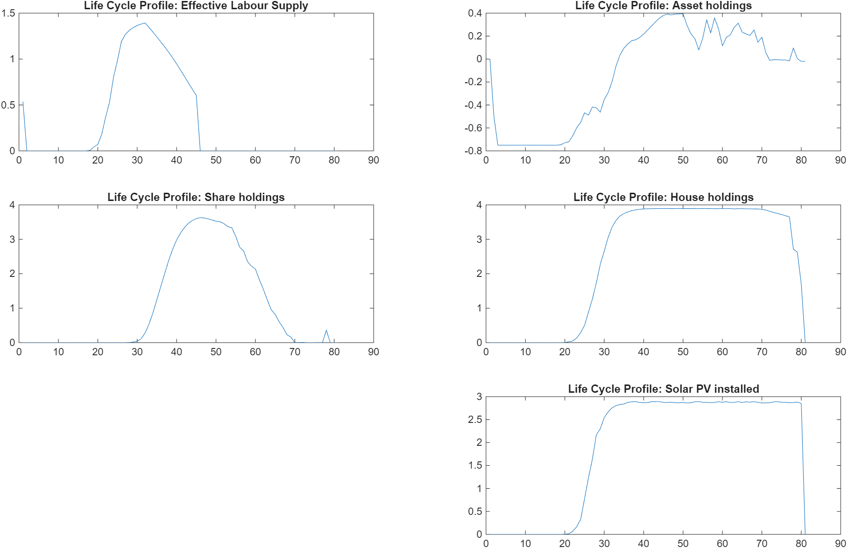
The extension to the model adds housing and solar pv panels to the household decisions about labor, leisure, and share-buying. Specifically, we add assets which allow an agent to take on a certain amount of cash debt (with a suitable credit wedge for loans vs deposits), choosing one of 5 types of houses (rental, and sizes 1, 2, 3, and 4), and solarpv capacity (0, 15kW, 30kW, and 45kW). solarpv is an experience asset that can be installed at house purchase time, or can be upgraded (with extra costs) at a later time. Once installed, it also degrades very slowly over time (creating later opportunities to upgrade).

n_d.household=[15,5]; % Decisions: labor, buyhouse
n_a.household=[11,11,5,4]; % Endogenous shares, assets, housing, and solarpv assets (0-45 kW generation)

%% To speed up the use of experienceasset we use 'refine_d', which requires us to set the decision variables in a specific order
vfoptions.refine_d.household=[1,0,1]; % tell the code how many d1, d2, and d3 there are

I wanted to model the fact that climate change will be irreversibly changing exogenous costs, such as energy costs and housing stock. And with the introduction of debt, I also needed to write rules so that agents could not take out loans to buy shares, only houses (and only to a certain amount).

On my system (with a 32GB GPU), the GE is solved (with loose tolerances) in 5347 seconds, or about 90 minutes. You can see that this model retains the various shocks (exogenous z and iid e) of OLGModel14.

The reported GE is:

Following are some aggregates of the model economy: 
Output: Y=    0.27 
Aggregate TFP: Y=    1.17 
Capital-Output ratio (firm side): K/Y=    1.28 
Total share+asset value (HH side): P*S (0.88) + A (-0.36) =     0.52
Total house value (HH side): H=    1.47 
Total bad debt (HH side): P*S=   -0.00 
Total firm value (firm side): Value of firm=    0.57 
Consumption-Output ratio: C/Y=    1.08 
Government-to-Output ratio: G/Y=    0.36 
Wage: w=    1.01

The VFIToolkit is amazing, and I’m looking forward to refining this model further as I learn more and talk with others who are interested in modeling energy transition economics within an OLG framework.

You can look at my repo here: GitHub - MichaelTiemann/OLG-Electrify: OLG model for electrification (Rewiring Aotearoa)

3 Likes

Congratulations! I agree with you that the VFI toolkit is amazing :slight_smile:

I had a quick look at the main script of your project on Github and I have noticed that you use grids with a small number of points:

Params.agejshifter=19; % Age 20 minus one. Makes keeping track of actual age easy in terms of model age
Params.J=100-Params.agejshifter; % Number of period in life-cycle
n_d.household=[15,5]; % Decisions: labor, buyhouse
n_a.household=[11,11,5,4]; % Endogenous shares, assets, housing, and solarpv assets (0-45 kW generation)
% Exogenous labor productivity units shocks (next two lines)
n_z.household=7; % AR(1) with age-dependent params
vfoptions.n_e.household=3; % iid
N_j.household=Params.J; % Number of periods in finite horizon

% Grids to use for firm
n_d.firm=31; % Dividend payment
n_a.firm=51; % Capital holdings
n_z.firm=11; % Productivity shock
N_j.firm=Inf; % Infinite horizon

Given the amount of GPU Ram at your disposal, you could increase the number of grid points for assets and labor (which are 15 and 11 respectively, unless I misunderstood). The number of grid points for firm capital seem relatively small as well.

Goo luck with your project!

1 Like

The number of grid points I’ve selected is based on maximizing the performance efficiency of the GPU. It’s true, the grids use only 50% of my available memory, but the GPU cranks away at 99% throughout most of the computation. As I slowly add gridpoints, GPU memory utilization increases. But also, the GPU utilization percentage drops, some due to increased “Copy” operations and some, I believe, due to increased “Shared Memory” usage. It is easy to land on 50% GPU utilization with still less than all GPU memory being utilized.

Increased grid sizes mean increased counts for iterations. Decreased GPU utilization percentage increases that by another factor. What I’m really hoping for is that in a few weeks we might have the code paths implemented to support grid interopolation with experience assets. That should give the best of both worlds.

In the mean time, I plan to look at the minimums and maximums of the state space used within the action space, and create smaller grid ranges that still allow for some reasonable excursion without giving up too much internal precision. I’m pretty sure that I’m still being very much too generous in terms of how many shares or how large the deposits and/or loans need to be.

Another dimension of opportunity is time. Right now periods are annual, so we have 80 such. That’s a large dimension in J, which contributes to both memory (in some cases) and iteration counts (in most cases). My model actually hybridizes LifeCycleModel35 (portfolio choice) with OLGModel14 (household and firm permanent types), before adding experience assets and other features.

LifeCycleModel35 has a few incarnations, including LifeCycleModel35semiz (in one of Robert’s personal repositories). The latter difference from the former by stacking up 5-year periods. I had a go at making the period length parametric (ranging from 3 years, which is the minimum for one of the Farmer-Toda calculations) and 15 years (which is the minimum to make visible the evolution of age-based wage evolution, kappa_j). The semi-endogenous shocks that its models greatly expands the state space, and my computer can handle 4-year periods by allocating an extra 200GB of swap to complement my 256GB of RAM. It can fit the 5-year model into RAM with minimal swap, and we see that performance scales as the inverse cube of the period size from there down to 15-year periods.

I’m very comfortable with period maths when it comes to simple exponential equations (such as computing that a 5% annual return is the same as a ((1.05^5)-1)% 5-year period return. But there are many other equations in OLGModel14 where I don’t know the identity tricks to compute more complicated and mixed annual recurrence relationships. But if there were a resource I could study for that (short of a year of maths), then crunching the model into 5 year periods would be really awesome (and make me feel less bad about suffering a 2x slowdown in a 2x larger problem resulting in a 4x overall time increase). For me, a 1-2 hour computation is manageable for making iterative daily progress.

2 Likes