On solving models with entrepreneurs

I’d like to share on the forum some simple thoughts on solving models with entrepreneurs. Examples of heterogeneous agents models with entrepreneurs are, among many others,

When solving these models with the VFI toolkit, one runs easily into memory problems since one has to define at least two decision variables d in addition to the standard endogenous and exogenous states. Typically, we have capital and labor demanded by entrepreneurs (Kitao 2008), or labor supply, capital and labor (Bruggeman 2021).

If the model is infinite horizon, one can solve for the steady state using the “refinement” option which essentially precomputes the optimal d before the VFI loop starts. This trick, however, is not available for transitional dynamics or more generally for finite horizon/OLG models.

However, in almost all cases that I’ve seen, one can easily derive the optimal values for k and n analytically (ok, not labor supply…), there is no need to use a grid. This is true as long as the entrepreneur’s after tax income is monotonically increasing in taxable income, which is almost always satisfied. I attach below a short note that I’ve written.

Let’s start with the original formulation of the entrepreneurs’ problem (essentially copied and pasted from Bruggeman 2021):

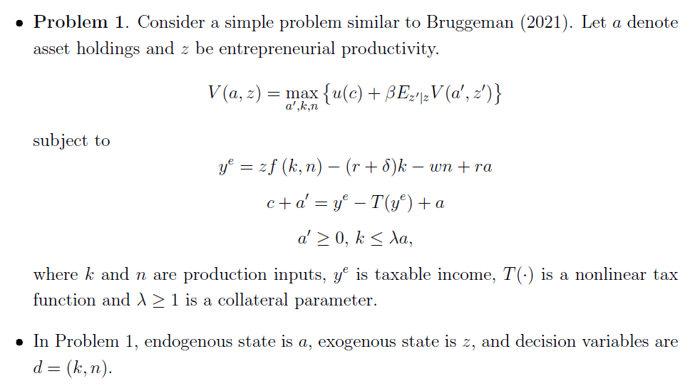
Toolkit: a is endogenous state, z is Markov exogenous state and d=(k,n) are two static decisions.

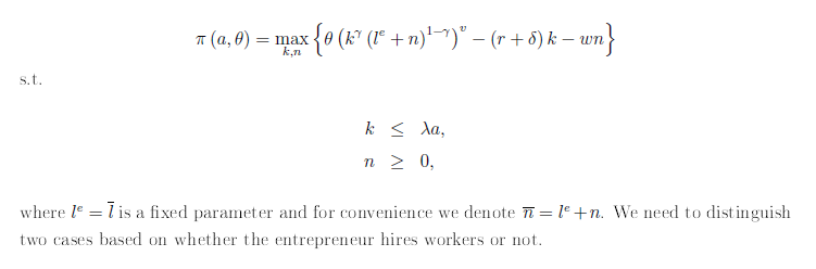
It turns out that the problem can be rewritten equivalently as:

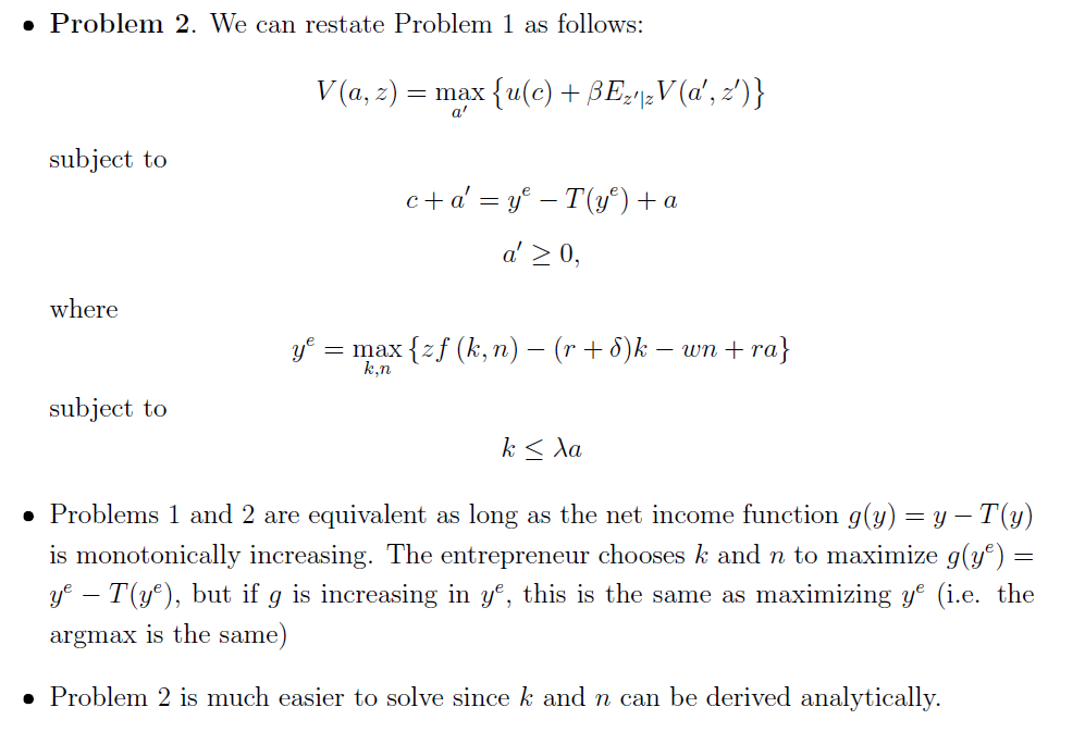
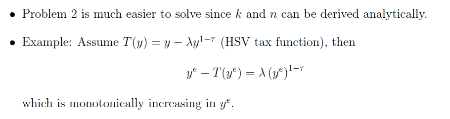
The attached text explains why. As an example, one can assume that T() is a progressive tax function as in Heathcote, Storesletten and Violante (XXX), but T does not have to be differentiable of course.

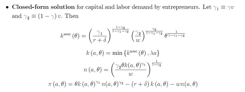
Why is this progress? Because we can derive k and n analyticaly, so they don’t have to be included as d variables. Let’s assume a functional form for the production function f(k,n) as below (basically, a decreasing returns to scale production function as in Lucas (1978))
image
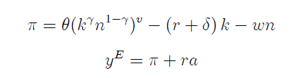
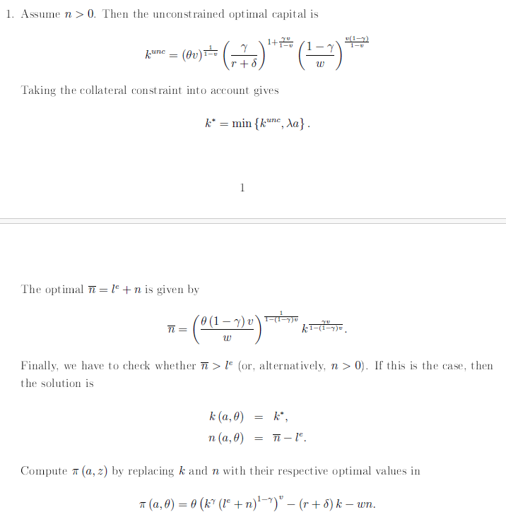
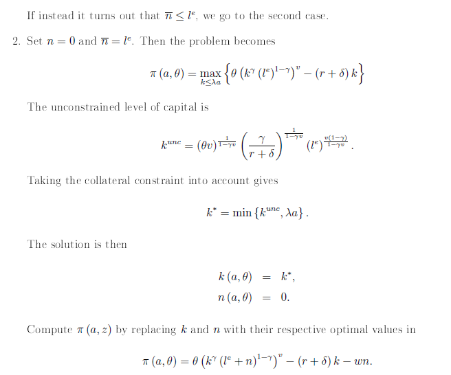
then we can take FOCs and obtain a closed-form solution:

Note: in my note above, assume that theta=z (entrepreneurial ability or productivity)

1 Like

I will update this post to include the case where the labor input used in the entrepreneurial production function is l^e+n, where l^e is fixed labor supply of the business owner and n is hired labor.
This is the case used e.g. in Bruggeman (2021).

There is a corner solution at n \geq 0. Entrepreneurs with low ability choose n=0 (there are NOT employers), so they use only l^e in production.

In the utility function, it is always l=l^e.

2 Likes

Here is the entrepreneurs maximization problem as in Bruggeman (2021). a is assets and \theta is entrepreneurial productivity.

First we assume that n>0, and we have the following:

Then we verify that the n we have found is greater than 0. If not, we have a corner solution at n=0.

I coded the closed-form solution in the function below.

function [profit, k, n, y] = solve_entre(a, theta, gamma, vi, r, w, delta, lambda, le)
%SOLVE_ENTRE Optimal entrepreneurial choices given a collateral constraint.
%
%   [PROFIT, K, N, Y] = SOLVE_ENTRE(A, THETA, GAMMA, VI, R, W, DELTA, LAMBDA, LE)
%   computes the optimal capital demand K, labor demand N, output Y, and
%   profit PROFIT for an entrepreneur facing a collateral constraint.
%
% INPUTS:
%   a      : Assets
%   theta  : Entrepreneurial ability
%   gamma  : Capital share in production
%   vi     : Span-of-control parameter
%   r, w   : Interest rate and wage
%   delta  : Depreciation rate
%   lambda : Collateral constraint parameter (k <= lambda * a)
%   le     : Fixed labor supplied by the entrepreneur to her own firm
%
% OUTPUTS:
%   profit : Optimal profit
%   k      : Optimal capital demand
%   n      : Optimal hired labor demand
%   y      : Optimal output
%
% ASSUMPTIONS:
%   Production function:
%       y = theta * (k^gamma * (le + n)^(1 - gamma))^vi
%
%   Profit to be maximized:
%       y - (r + delta) * k - w * n
%   subject to:
%       k <= lambda * a
%       n >= 0
%
%   The function first solves the unconstrained problem assuming n > 0,
%   then checks whether n > 0 is feasible. If not, it re-solves imposing n = 0.

%% Case 1: Unconstrained solution with n > 0

% Unconstrained level of capital (n > 0 candidate)
aux1   = (gamma / (r + delta))^(1 + (gamma * vi) / (1 - vi));
aux2   = ((1 - gamma) / w)^((vi * (1 - gamma)) / (1 - vi));
k_unc  = (theta * vi)^(1 / (1 - vi)) * aux1 * aux2;

% Apply collateral constraint
k_star = min(k_unc, lambda * a);

% Compute n_bar = le + n from FOC for labor
exp1   = 1 / (1 - (1 - gamma) * vi);
n_bar  = (theta * (1 - gamma) * vi / w)^exp1 * k_star^(gamma * vi * exp1);

%% Check whether n_bar > le (i.e. n > 0)

if n_bar > le
    % Constraint n >= 0 is NOT binding
    k = k_star;
    n = n_bar - le;

else
    % Case 2: Re-solve imposing n = 0  (so le is the only labor input)

    aux1  = (gamma / (r + delta))^(1 / (1 - gamma * vi));
    aux2  = le^((vi * (1 - gamma)) / (1 - gamma * vi));
    k_unc = (theta * vi)^(1 / (1 - gamma * vi)) * aux1 * aux2;

    % Apply collateral constraint
    k_star = min(k_unc, lambda * a);

    k = k_star;
    n = 0;
end

%% Output and profit (same formulas in both cases)

y      = theta * (k^gamma * (le + n)^(1 - gamma))^vi;
profit = y - (r + delta) * k - w * n;

end % function solve_entre

1 Like