For those following this thread, I have an update, and a request for feedback.
I managed to find what I think is an elegant way to integrate AggVars into PTypes so that they feed forward without duplicating any calculations or otherwise disturbing the flow of the system. It allows me to continue to use the CMA-ES solver, and it solves faster than ever, because I’ve eliminated a pricing variable that is truly unconstrained (dividend price expectation).
But that revealed a few more things about my model’s return function for firms (based on OLGModel14_FirmReturnFn.m):
function F=OLGModel14_FirmReturnFn(dividend,kprime,k,z,w,delta,alpha_k,alpha_l,capadjconstant,tau_corp,phi,tau_d,tau_cg)
% Whether we set it up so that dividends or equity issuance is the decision
% variable is unimportant, here I use dividends as the decision variable.

% Note: r is not needed anywhere here, it is relevant to the firm via the discount factor.

F=-Inf;

% We can solve a static problem to get the firm labor input
l=(w/(alpha_l*z*(k^alpha_k)))^(1/(alpha_l-1)); % This is just w=Marg. Prod. Labor, but rearranged

% Output
y=z*(k^alpha_k)*(l^alpha_l);

% Profit
profit=y-w*l;

% Investment
invest=kprime-(1-delta)*k;

% Capital-adjustment costs
capitaladjcost=(capadjconstant/2)*((invest/k-delta)^2) *k;

% Taxable corporate income
T=profit-delta*k-phi*capitaladjcost;
% -delta*k: investment expensing
% phi is the fraction of capitaladjcost that can be deducted from corporate taxes

% Firms financing constraint gives the new equity issuance
s=dividend+invest+capitaladjcost-(profit-tau_corp*T);

% Firms per-period objective
if s>=0 % enforce that 'no share repurchases allowed'
    F=((1-tau_d)/(1-tau_cg))*dividend-s;
end

% Note: dividend payments cannot be negative is enforced by the grid on
% dividends which has a minimum value of zero

end
As discussed elsewhere, in this particular case, when tau_d is equal to tau_cg (both are set to 0.2), the ratio ((1-tau_d)/(1-tau_cg)) is 1. And when we look at dividend-s we find that because s is dividend+invest+capitaladjcost-(profit-tau_corp*T), the subtraction makes dividend irrelevant to the objective function, other than that it governs the feasibility of share issuance (s>=0). By plotting a 3D surface with x,y axes of dividends vs capital (K) and F in the z axis we can confirm that where F is not -Inf all values along the dividends axis are equal.
By feeding the actual offered dividend into the household function (rather than using a GE price that’s trying to track this largely untethered dividend value), the solver quickly steered into a very opinionated direction by optimizing this equation (the rewrite with dividends removed):
F=profit-invest-capitaladjcost-tau_corp*(profit-delta*k-phi*capitaladjcost)
That equation was optimized by using the smallest amount of labor and capital possible, and perhaps benefiting from a rounding error caused by the grids. That doesn’t inspire a lot of confidence in capitalism!
I used to be the CEO of a company, and my bonus used to be based on a combination of metrics, including revenue, profitability, and maintaining financial covenants. Here’s where I’m interested in your feedback. I added this term, intended to steer the company’s behavior to something a CEO would realistically decide:
y*(1-(dividend-0.2)^2)/10
The rationale is
- We want firms producing output, so Y is valuable
- We want firms aiming for a reasonable dividend payout rate, so square of the difference of a market target that’s meaningfully higher than the rate of risk-free return.
- We want these goals to steer, but not dominate, the overall return function based on profits, investments, etc. Alas, we cannot normalize Y to be profit-sized, because Y*(1/Y) defeats objective #1. I found by trial and error that once we divided by 10, the solver could meaningfully walk through the action space. Indeed, it initially started with a guess of using almost all the capital and paying a liberal dividend, but it quickly (in fewer than 10 iterations) ramped down to a dividend rate close to 20%, and labor and capital coming into line with household and other expectations (like CapitalOutputRatio).
I found that when dividing by less than 10, the solver insisted on using the absolute maximum capital the grid would allow and demanding more labor than households were able to supply.
So the whole return function calculation becomes:
F=(((1-tau_d)/(1-tau_cg))*dividend-s)+y*(1-(dividend-0.2)^2)/10
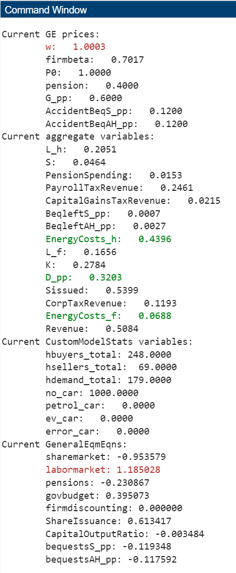
This leads to the following aggregate outputs (when there are no z and e shocks):
Following are some aggregates of the model economy (Scenario 1):
Output: Y=    0.40
Aggregate TFP: Y=    1.00
Capital-Output ratio (firm side): K/Y=    2.20
Total share value (HH side): P*S (1.10) =     1.10
Total firm value (firm side): Value of firm=    1.12
Consumption-Output ratio: C/Y=    2.03
Government-to-Output ratio: G/Y=    0.11
Wage: w=    1.00
Which look very reasonable. I’ll update when my run using z and e shocks complete.
In the meantime, the feedback I seek is this: how should one think about the balance of using very general equations (such as “maximize profits”) to find equilibrium solutions, vs. injecting behavioral opinions (such as “maximize profits while producing products and paying shareholders”)? Where is the line between discovery and self-fulfilling prophesy? Or, is this a case of saying “Lo, I have discovered good advice for both economists and capitalists: use THIS as an objective function and you’ll find both market pricing stability and satisfactory strategic behavior”?