Lifecycle analysis provides an opportunity to calculate optimal choices for consumption, investment, leisure, and bequests, even (or especially) in the case of uncertainty. That being said, I have also come to understand that humans tend to save more than their optimal agent counterparts would, leading to an excess of “Accidental Bequests”. The VFIToolkit lifecycle model can balance the lifetime utility function books by calculating a warmglow of bequest to make agent behavior match human behavior.
Members noted risks regarding the speed of the economic recovery. The Committee noted the risk that household spending could be slower to recover than currently assumed, particularly if house price growth remains subdued. This could lead to households continuing to maintain higher levels of precautionary saving. Conversely members noted a risk that higher export incomes and the return of capital to dairy farmers from the sale of Fonterra’s consumer brands business could spur higher investment and consumer spending by farmers.
Are there papers that quantify the economic cost, inefficiency, and/or instability risks of reserve banks fighting against skeptical consumers who save too much?
Any model with incomplete markets will generate precautionary savings, which includes essentially all the models that VFI Toolkit solves. E.g., in any of the OLG models with idiosyncratic shocks, there is no asset that ‘spans’ the space of outcomes (the only asset is savings, and the return to your savings does not depend on your personal idiosyncratic shock), so these are incomplete market models. In the Intro to Life-Cycle Models there are a few examples that illustrate/explain this in more detail (models 15-19).
If ‘risk’ increases, then the precautionary savings increases, which is what the bold sentence in your post is essentially describing. So then you just need a way to change the level of risk. The most common approach is to have ‘uncertainty shocks’, which is a shock that, e.g., takes two values low and high, when the uncertainty shock is low the idiosyncratic shocks are smaller, when the uncertainty shock is high the idiosyncratic shocks are larger. In most applications you would want the uncertainty shock to be an aggregate shock (so it impacts everyone in the economy), and you can also have market incompleteness in respect to aggregate shocks; you would likely also add, e.g., aggregate TFP shocks whose variance depends on the value of the aggregate uncertainty shock.
Standard HANK models look at monetary policy in the presence of precautionary savings. But this is not the same as ‘higher levels’ of precautionary savings. I’ve not seen anyone solve a HANK with uncertainty shocks and think about optimal monetary policy in response to increases in precautionary savings; likely no-one has as 90+% of HANK models get solved under linearization so you cannot think about this question in them. There is a small but non-zero chance someone has look at this, a google around suggests two 2025 papers are trying to start on this, but both are not really there yet: Modeling uncertainty in HANK models - e-axes. [Uncertainty shocks and monetary policy in RANK models has been done (presumably), but you don’t really have precautionary savings there.]
PS. HANK=Aiyagari+Aggregate shocks+Sticky prices
PPS. I have only seen one HANK paper with life-cycle, that is one HANK-OLG, no doubt more are coming out this year as that is just entering the realm of ‘things we can solve’.
PPPS. “Arrow-Debreu Securities” is the technical term for assets that span the space of outcomes, and that are needed for markets to be complete.
A minor point about the definition of HANK: I think having aggregate shocks is not essential. In the seminal HANK paper by Kaplan, Moll and Violante,
there are no aggregate shocks. The authors study the response to shocks with MIT shocks (i.e. what the toolkit does with the transition command in infinite horizon).
I would define HANK as a New Keynesian model with incomplete markets.
half agree, but the transition path is intended to be interpreted as an IRF to an aggregate shock [at the time when they wrote the article this was hand-waving, but has since been formalized by BKM]
So in the end they are doing the linearized solution to a model with aggregate shocks (same as SSJ, just they only half-exploit the linearization while SSJ fully exploits the linearization). It is coincidence that this happens to look exactly the same as solving a transition path in a model without aggregate shocks.
Very much appreciate the references and discussions around this topic–thanks! Let me make it more concrete: in the case of energy transition from fossil fuel to rooftop solar (which could be on a house, a school, a community center, etc), electricity goes from being an expense to an endowment. So here’s a list of thought experiments:
Household Agents source energy either from conventional supply (that delivers gas, electricity, and petrol) or from abundant rooftop solar that meets >= 90% of their daily needs, and can meet 100% of their needs averaged over two weeks. We want to model (as simply as possible) agents who go about their lives working, consuming, and investing as usual, and whose usual behavior supports firms and funds government services (OLGModel14 comes to mind). Using a parameter that evolves gradually over time (perhaps using Transition Paths), agents switch from 100% conventional supply to 100% rooftop solar. We don’t concern ourselves with the cost of that conversion, only the question of how shocks affect those who are conventional fuel users vs. those who are rooftop solar users. In particular, how energy shocks affect precautionary savings and consumption, and how that affects demand, firm profitability, investment, taxes, pensions, etc. We don’t concern ourselves with how firms are otherwise affected by the shock other than by consumer demand.
In the second case, we look at shocks from the firms’ perspective. In this case, energy cost factors into profits and energy availability factors into total factors of production. Our firms produce goods that can be classified as “essential” (low elasticity of demand) and “non-essential” (higher elasticity of demand). We should see firms producing essentials raise prices (to maintain profits) while firms producing non-essentials cut back production and profits. We can then similarly use a parameter (perhaps using Transition Paths) to evolve over time the percentage of firms (of both types) that can source energy from conventional or self-generated supplies (electrified truck fleets and manufacturing facilities, etc). We don’t concern ourselves with changes to household energy sources, but we do concern ourselves with households that become unemployed due to lack of demand. And we are interested in firms’ sensitivities to shocks.
In the third and final case, we can use a parameter in both household and firms, creating four (or perhaps eight) cases: conventional vs. solar households employed by conventional vs. solar firms (perhaps making essential vs. non-essential goods). These similarly evolve over time from 100% conventional to 100% solar-endowed. How do the equilibria of these four (or eight) cohorts change across the transition, and how sensitive are they to shocks?
Any thoughts on the difficulty of making simple models credible out the outset vs. what they might teach us about the effects of precautionary savings under their simple assumptions? I suspect we will find that the conventional households working for conventional firms will fare worst, and the solar households working for solar-powered firms will fare best, but by how large a margin relative to the shock function–that’s the question.
Regarding the above, would it be more accurate to say that this observed tendency is related to a natural “Ambiguity Aversion” (maximizing the worst possible future) rather than blaming human imperfection in attempting to maximize the most likely future (as optimal value function iteration allows us to do)?
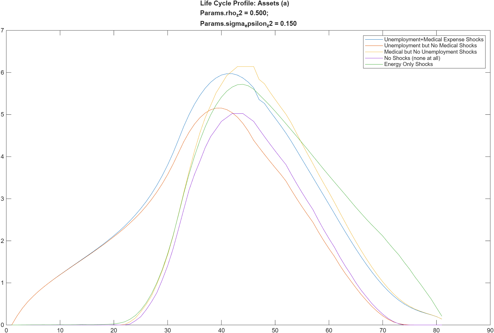
Unemployment shocks cause greater precautionary savings early in life, when unemployment risk is higher.
Medical expense shocks cause greater precautionary savings later in life, when risk of health problems is greater.
The purple line shows “no shocks (at all)”, showing what is the ideal level of precautionary savings (maximizing consumption and leisure (both!) through until death).
The green line shows what happens to “no shocks” if, indeed, there is an AR(1) energy shock affecting 1/3rd of the agents’ budget, with the expectation that the result of the shock is 50% higher energy pricing. Why 1/3rd of the budget? That’s the energy-related expenses of a “living wage” agent in NZ (which is much more than just utilities, it also includes a chunk of transportation, and other essentials). The 50% higher fuel price is a likely outcome of the 100% increase in oil prices to an economy that derives 55% of its energy from fossil fuel.
This teaches that precautionary savings in the face of fuel shocks really ramps up when heading into retirement. Which is probably why the 65+ crowd is so vocal about fuel prices.
Please feel free to comment on the AR(1) parameters I used.
My (admittedly weak) understanding is that distinguishing risk aversion (expected utility, with concave utility fn) from ambiguity aversion (utility under worst possible future; max-min utility) is very difficult. My impression based on what little I have read of the literature is that it is better to think of people’s expectations with regard to different sources of uncertainty as risk or as ambiguity. So peoples expectations with regard to their income next year might be treated as risk, while peoples expectations with regard to AI might be treated as ambiguity (I made the later example up on the spot). This seems to better capture behaviour that saying ‘people are risk averse’ or ‘people are ambiguity averse’ as two strictly exclusive categories.
In basic life-cycle models the more likely cause of ‘excess’ savings [data has more savings than model] at older ages is a bequest motive. This is what the ‘warm-glow of bequests’ is attempting to model in a parsimonious way. [If you actually model bequests based on ‘parent’ getting utility in proportion to the utility of their ‘child’, then you get a game-theory problem as the child knows they will be given bequests and changes their behaviour in response, so parent wants to give a generous bequest to child, but also doesn’t want the bequest to be so generous that the child become indolent. The use of ‘warm glow of bequests’ allows up to attribute this motive to the parent without having to deal with game-theory.
The other main contenders in the literature for large savings by the elderly (other than bequests) are to pay for large health expenses (possibly nursing homes).