This paper came out in EER today, I downloaded it and built the main model. Codes on github. Life-cycle model solves in about 3min on my desktop, so GE takes a few hours. If you have access to a high-end server GPU it will be fast enough that you could do the full replication over a weekend (requires solving the general eqm problem maybe 60 times, on a grid for two UI parameters).
Some minor differences from original:
they have a closed-form solution for search effort, ‘s’, but toolkit cannot exploit it so I use 11 points
they use a discrete grid on labor effort ‘n’, I use 11 points but don’t know how many they use
they have n_a=50, I use 150
Main purpose of this was just for me to test for myself what is possible with Claude + VFI Toolkit.
Note: VFI Toolkit can solve this model because it is ‘search labor’ (exogenous job-finding probability), but cannot yet solve ‘search and matching’ (endogenous job-finding probability).
You mean that the model in partial equilibrium takes 3 minutes but in general equilibrium takes so long? I didn’t realize the state space is particularly large.
I realize now that there are really many periods in the lifecycle, perhaps because the calibration is monthly/quarterly. So the state space is indeed larger than usual, and the age dimension cannot be parallelized.
Q: Is the run time you report based on grid interpolation? Maybe one could speed things up by using pure discretization to find (get close to) the general equilibrium.
Good point. I wonder if there is a “clever” way to let the toolkit skip the shocks in retirement, without writing 300 additional functions I mean.
In some of my codes I use nz_help dependent on age. The logic:
If j<Jr
nz_help = n_z (does all points)
Else
nz_help = 1
End
Then nz_help is passed to the value function routine. Value function and policies are still defined on the full grid [n_a,n_z,J].
The problem in writing a general toolkit routine is that not all z shocks are equal: health shocks or medical expenses shocks, for example, are present during the whole life-cycle, while productivity shocks only during working age. It looks complicated. Maybe Fable 5 can help (when Trump decides to restore access to it).
Another inefficiency in solving this model with the toolkit, which is unrelated to the one above: what about search effort if the agent is already employed? I think in the model there is no on the job search, so when employed the optimal search effort is trivially zero, but the toolkit still loops over all possible values for search effort. Is it possible to design the grid for search effort so that it is the full grid when the semiz=unemployed but only one point when semiz=employed?
The easy trick that the toolkit can already do is that none of the UI policies in the loop impact retirement at all. So you can just solve once, then keep the period Jr (first retirement period) value fn, and then set vfoptions.V_Jplus1=V(:,Jr) and N_j=Jr-1 and use that in the loop.
[V_Jplus1 is not well tested, so would be worth running once to check it does give same answer under same policies]
This essentially removes retirement completely from the problem (after you solve it once), and so would slash runtimes about 1/3 (as roughly 1/3 of periods are retirement).
Note that this is better than anything you can do with n_z differing by age. But it is not a trick that works in most models.
[I think this is correct, I did not look closely at exactly if there is no impact on retirement when changing UI policies in the loop, because I didn’t attempt to code that loop.]
The reason is that the closed-form solution for search effort depends on the value functions in the next-period, right? So the cost of search effort occurs today while the benefit is encoded in the value of being employed tomorrow relative to unemployment.
Technically, the toolkit can use a closed-form solution for a decision variable as long as it can be written inside the current reward in f_ReturnFn, and obviously f_ReturnFn does not allow value functions as input arguments.
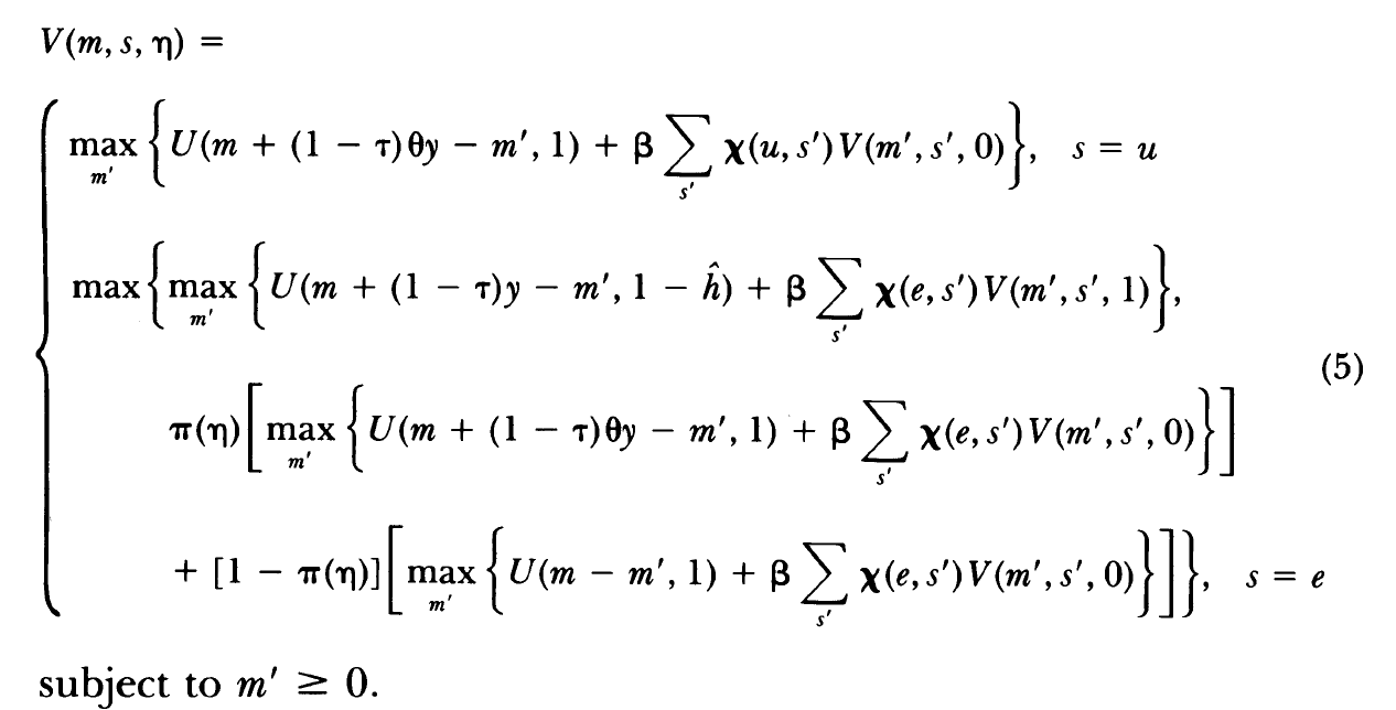
I thought it would be easy for the toolkit to replicate this older paper, but I am not sure how to treat the state variable \eta in the paper. To explain the setup:
a is endogenous state, assets
s \in \{u,e\} takes two values, unemployed and employed, and is an exogenous Markov state.
\eta is a state variable equal to 0 if the agent did not work in the previous period and equal to 1 if the agent worked.
An agent starts the period with assets a and employment opportunity s. If s=u, he is not given an opportunity to work, earns unemployment benefits \theta y and chooses savings a'. If instead s=e, he is given an opportunity to work. He can then choose to accept it and in that case he earns the wage y. If he chooses to reject it, the government will audit him and he will receive benefits with probability \pi(\eta) or be punished and receive nothing with probability 1-\pi(\eta).
I am not sure how to define \eta for the toolkit. It could be a second, discrete endogenous state variable but where to define \pi(\eta)? Or I could introduce a decision variable d for work vs not work.
Here is the Bellman equation. Note that I redefined m as a.
You can get close to Hansen & Imrohoroglu (1992), but not quite. The problem piece is that the whether or not you get unemployment benefits if you ‘lie’ is a probability that is determined during the same period (you could easily implement if it resolved next period, which would work just fine in a higher frequency model, e.g., if you made the time period monthly or weekly).
The state space of the model in their notation is V(m,s,\eta), which in toolkit notation can be done as V(a,z,semiz). The assets (m) are a standard endogenous state; the ‘employment opportunity’ (s) is a standard markov state which takes just two values (e and u); the ‘worked last period’ (\eta) is a semi-exogenous state which takes just two values (0 and 1). There is only one decision variable h (which takes just two values, 0 or \hat{h}), and this determines the evolution of the semi-exogenous state.
The one piece of the model that does not work is that if you choose h=0 when you have an employment opportunity s=e then with probability \pi(\eta) you get a benefit and with probability 1-\pi(\eta) you get a penalty. The difficulty is that this probability has to be resolved during the period (the dependence on \eta is a non-issue). VFI Toolkit presently has no way to do this.
If you instead had a higher frequency model you can imagine that if you choose h=0 with s=e you could get get the benefit this period, but then with some probability next period you get banned from receiving any benefits for the next five periods and have to pay a fine. This would be implementable.
PS. Technically you could implement it in VFI Toolkit by having an additional two value markov that is the ‘sub-period’, so you choose h=0 with s=e in first sub-period, then between period shock decides benefit or penalty, and you then enter second sub-period. This would work and allow you to solve the model with toolkit, but it will be about twice as hard a problem as you actually need to solve, so not worthwhile.