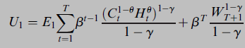
I am interested in modeling the effects of housing on the demand for risky assets. I am looking for code that replicates models similar to Cocco (2005). In this paper, consumption within the utility function is divided into nondurable goods consumption, denoted as Ct, and housing consumption, denoted as Ht, as follows:
Is it possible to handle such problem by combining available VFI Toolkit life-cycle models? Could you please assist me with your suggestions?
[Edit: two years later, there is a code implementing Cocco (2005) further down this thread. ]
I leafed over the paper. Unless there is a trick I am missing this model has two endogenous states: assets and housing. In principle the toolkit can do this but in practice it will be too slow to be of any real use
He makes each model period 5 years, so doesn’t have to solve many periods. This helps.
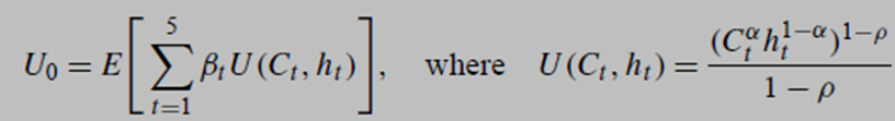
Housing has a dual meaning here. Homeowners receive utility from its consumption services and also return from its investment if the house were to be sold. I plan to introduce only 5 periods, similar to Hu (2005) in 'Portfolio Choices for Homeowners’ published in the Journal of Urban Economics:
In Cocco paper there are two (but read below) endogenous states: asset holdings a and housing h but in practice the second state (housing) is discretized using few grid points. However an extra complexity is the choice of renting vs owning, so in principle you have three endo states: (a,h,o) where o is a dummy for housing tenure.
Update: it seems there is no renting choice in Cocco (2005)
I think the code would work just fine for 5-10 periods, portfolio-choice plus housing, and in my head I can see how to implement it. If I can find some spare time in the next 1-3 months I will put it together. Hopefully, but no promises [Is just a matter of combining the risky endogenous state, which is currently Case3, with a standard endogenous state. Easy given that each is already done seperately, just will take a few days to code and debug.]
You can typically avoid having a whole state for own/rent. The trick is to have one of the points on the housing grid be zero, and simply assume that everyone who does not own any housing rents. You can then assume that housing and consumption are joined together by a CES function, and so the split can be analytically derived, thereby avoiding computing renting altogether (it is modelled, but it does not meaningfully complicate any of the computations). [I’ve solved a model with housing before, hence why I know this trick ]
[Correction: Zach points out in comment below that the calibration used by Cocco (2005) as the baseline means this post is not actually correct for his baseline model.]
I went and read Cocco (2005) in detail. VFI Toolkit will easily do everything but one piece of the model. Specifically, Cocco (2005) has the risky asset returns shock (i.i.d. between period shock) correlating with the innovations to the earning shock (markov shock).
VFI Toolkit allows two shocks of the same type to be correlated, but it does not permit shocks of different kinds —here a u shock and a z shock— to be correlated.
You could do a workaround and model both as z shocks, and then do two endogenous states instead of the riskyasset, and this would work in the toolkit but would be rather wasteful. In some sense, the issue is that the is a ‘missing’ aggregate shock, which is the motive Cocco (2005) gives for the shocks being correlated.
So everything else in Cocco (2005) will be easy with VFI Toolkit, but a full replication is not possible because you cannot correlate the u and z shocks (the between period i.i.d. shock and the markov shock).
I am (attempting) to replicate this model and am not sure what you mean. I thought Cocco has perfect correlation between the housing and labor market shocks, and assumes zero correlation between the stock market and labor market shock:
”The correlation between innovations to aggregate labor income and innovations to stock
returns is slightly positive in the data, and equal to 0.047, although not statistically different from zero. Therefore, in the baseline case, I set it equal to zero”
Cocco (2005), page 540 says “I allow innovations in log returns to be correlated with innovations to aggregate income shocks (and house prices), and denote the corresponding coefficient of correlation by \rho_{\epsilon,\iota}.” where \epsilon is the innovation to \eta (eqn 4; pg 538) which is the aggregate labor income shock, and \iota is the shock to stock returns (eqn 8; pg 540).
I read this and just stopped there. I never read the actual calibration in detail since I could see in the equations that I couldn’t do a nice clean solution.
But as you say, later in the calibration section on page 547 there is the quote you point to that says "The correlation between innovations to aggregate labor income and innovations to stock returns is slightly positive in the data, and equal to 0.047, although not statistically different from zero. Therefore, in the baseline case, I set it equal to zero”. Based on this \rho_{\epsilon,\iota}=0, in which case VFI Toolkit can solve it just fine as a ‘riskyasset’.
I just never read that far Thanks for pointing this out. So at least the baseline model should be implementable just fine with VFI Toolkit.
Yes I don’t believe he ever experiments with that parameter in the manuscript. If anyone indeed is preparing to replicate this model with the toolkit, I believe I can be of some assistance with the values/scalings of input parameters.
I would be very interested to see if the VFI toolkit can replicate the results of this model, even qualitatively, as I am unable to match them (I just have had no chance to try myself yet…).
I started working on Cocco (2005) codes. I have most of it down, other than a few remaining parameters.
I have one main unknown: can you have housing=0, and if yes, how does the utility function handle this?
Normally in a model with housing you would have “housing services” in the utility fn, not “housing” itself. And then renters (people with housing=0) can rent housing services for some rental price. But Cocco (2005) seems to say nothing about this, not even if H=0 is possible or if everyone owns houses, nor does he say anything about the grid on housing (other than that Hmin=20000), so unclear how many points and what the max house size is?
My guess is that he just does not allow the possiblity of H=0?
In which case, anyone have any idea what the grid on H should be? Is going to be hard to get the replication close to the original without a somewhat similiar H grid (it will only be a few points, so they are likely to matter).
I tried the minimum of the grid as 20,000, and added a point at 0 only for year 1. To the best of my knowledge, they all must purchase houses in the first period “there is no initial level of housing” (page 541). This means the model has some strange properties in the first period (default if the grid for the income process is dense enough - I think it should be three points however). Individuals are always forced to choose above the minimum, but can start at 0. Individuals cannot rent. It is likely he used either two or three points on the grid.
I think since the utility function contains a cobb douglas aggregator, you will have an interior solution for both inputs.
I had a look at the paper and Cocco (2005) considers only owned housing, no renting allowed. See e.g. footnote 7 in the paper. So H=0 is of course not allowed
The model runs just fine (<1min on my desktop, GPU has 8gb memory). Could do with a few more grid points on n_d(1), n_d(2), and n_a(3), but everything else seems enough (I believe everything else already has more points than the original); probably won’t change anything much but would be good regardless. If you had a powerful GPU you could not only increase the grid points, you could also turn off vfoptions.lowmemory which would make the whole thing vastly faster.
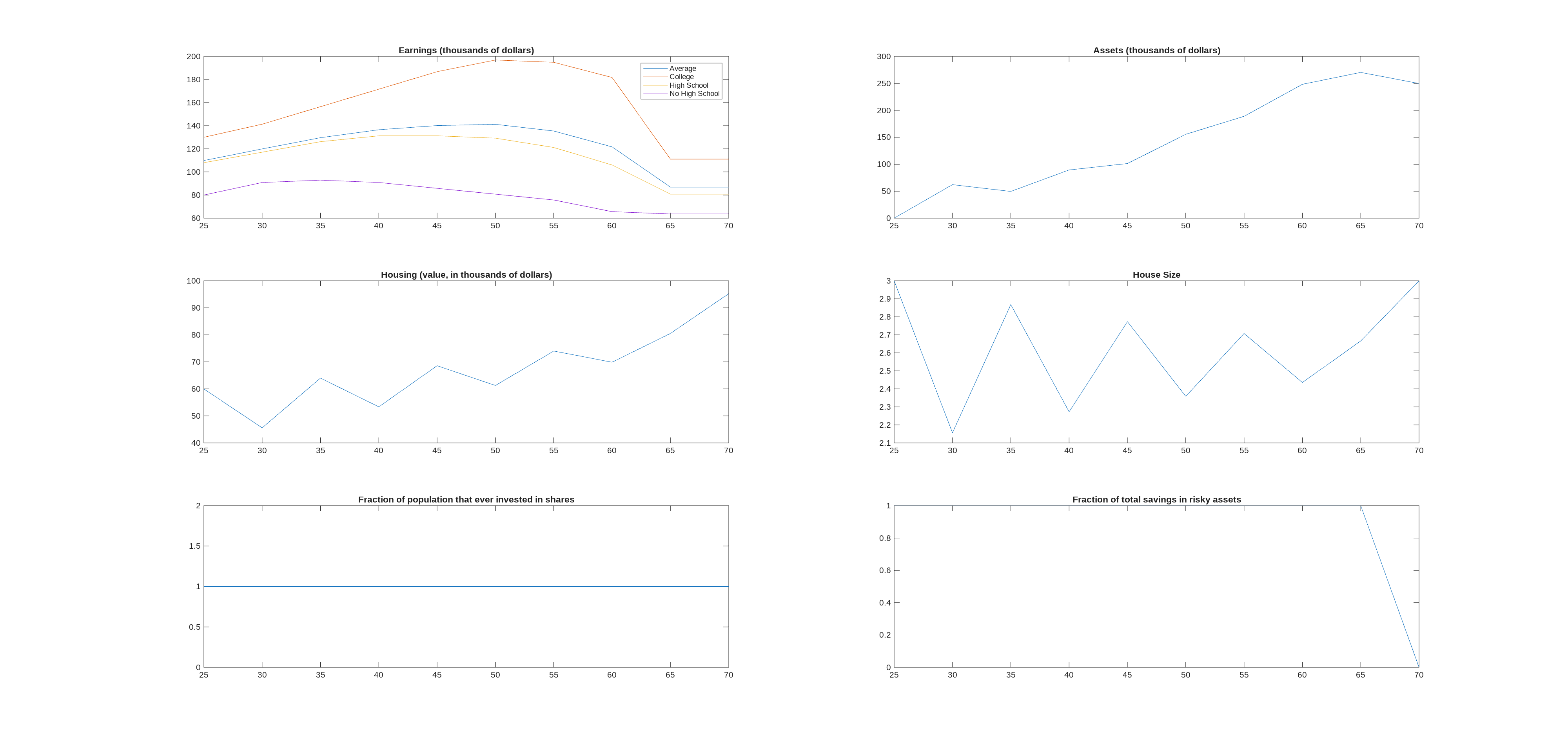
There is one important failing, and that is that everyone always does all their savings in the risky asset. I believe this is a problem with model rather than codes. By which I mean it follows from the calibration of the model. I did two tests of the codes, the first was to just make the return to risky assets worse than the safe asset (u_grid=0.9*Params.r_f*ones(n_u,1)) so risky share should always be zero (as risky asset is dominated by safe asset). Second test was to put
if sp==1 && agej<6
    F=-Inf;
end
in ReturnFn so no-one will invest in risky asset during first 5 periods. Both tests make the graph at end of the share of total assets invested in the risky asset do exactly what they should (zero for first test, zero in first five periods for second test).
Obviously it is possible my code has a typo, or I get one of the calibrations wrong (C2005 is pretty vague on some details of the model, so you are just kind of guessing for a few of the parameters).
The Cocco (2005) paper is missing a bunch of details about how the grid on housing was set, so I am largely guessing the grid, which could be part of the issue.
Apparently the original codes have been lost so no way to know if this is part of the issue, or was an error in the original code.
Note this model uses a low risk aversion (CRRA parameter gamma=5) for norms of the life-cycle portfolio choice literature [CGM2005 uses 10; it would be high by norms of the Macro literature, but this is portfolio-choice so that is the relevant literature.]
The following graph, produced by the codes, shows what is wrong with the risky share (for anyone who wants to see it but doesn’t have Matlab+GPU to run the codes).
PS. Part of the reason it wants more grid points is that you cannot yet use vfoptions.divideandconquer and vfoptions.gridinterplayer for riskyasset. With these the model would easily solve faster and to sufficient accuracy.
PPPS. Given the model solves so fast, could easily use the calibrate life-cycle model command to fix these issues, given some empirical targets to hit.
Nowadays I find one day is plenty to code models where the toolkit already has all the needed features. That said, it often then takes me 1-10 days more to track down the last few parameters that the paper does not really explain, or how to set the initial distribution of agents, or the grid on housing, or some counterfactual exercise that wasn’t spelled out in detail, etc. Since your codes gave me most of these I could dispense with the extra and keep it to one day
I originally had n_a(1)=6 (number of points in housing grid), and with this people just kept upsizing their house as they aged, so assets hardly increased over their life. Cutting it to n_a(1)=4 meant they max out housing and then save lots of assets towards end of life. This makes sense, and just tells us people in the model really love housing.
This still left that the mean house size (conditional on age) fluctuates slightly up and down. I tried adding the following lines at end of ReturnFn,
if abs(hprime/20000-2)<0.01
    if rem(agej,2)==1
        F=100; % odd ages choose hprime=40000
    end
elseif  abs(hprime/20000-1)<0.01
    if rem(agej,2)==0
        F=100; % even ages choose hprime=20000
    end
end
which should mean they choose house size 1 at even ages and size 2 at odd ages, and this was exactly what happened, so code seems fine.
I can imagine a story where the growth in prices over time, interacted with the collateral constraints, creates the kind of up/down in the house sizes. But it feels like I am just making up a story ex-post to justify what I see. So I’m still not entirely convinced of the housing, the wiggling up and down does seem weird.
Yes the wiggling to round numbers seems weird if this is indeed an average from simulations (especially given the transaction costs)?
In terms of the parameterization: I think annual HP growth should be annually 1% not 1.6% according to his comment at the end of page 545. I am also confused about the scaling of some parameters:
The code seems to use 0.03 (the annual amount) for the moving probability. And the return processes do not seem to have been scaled to five year levels (at least from lines 158 -163 of Cocco2005.m. I apologize if I missed something.
Edit - in fact - if leverage makes housing investment particularly attractive (and the returns on alternative assets should be scaled up) then perhaps this would generate the behavior you observe as households cash out their home each period and then leverage up.
You are right, I need to change some of those parameters from annual to five year. I am away until Monday so will have to wait until then.
As well as the returns (r_f, r_d, mu) and prob of moving (pi) I probably also need to adjust the standard deviations of shocks to be five year period.
For annual HP growth, Table 1 says “Real house price growth” denoted “b” is 0.016. Which matches with what what he uses “b” to denote in the paragraph just before eqn (6) on page 539.
On pg 545 is the quote you mention “During this period, log real house prices increased an average 1.59% per year. Part of this increase is probably due to an improvement in the quality of housing, which cannot be accounted for using PSID data. Therefore, in the simulations, I decided to use a lower value for the average annual increase in house prices of 1%.”
Based on this I am going to follow your suggestion and set b=0.01 (annual, so to the five year version of this in model), overruling Table 1 on the basis of this paragraph from pg 545.
How to convert the annual std dev to five yearly std dev?
The lazy approximation is to multiply the annual std dev by sqrt(5), apparently this is widely used as a rule-of-thumb approximation. But it is biased, since it assumes that returns are summing over time, and ignores the effect of compounding that occurs in reality.
To make things easier, let’s pretend we are converting monthly to annual. So we have the monthly standard deviation, \sigma_m, and we want the annual standard deviation, \sigma_a. The (incorrect) rule-of-thumb would be \sigma_m=\sqrt{12} \sigma_m, as there are 12 months in a year.
The correct formula is instead, \sigma_a=\sqrt{(\sigma_m^2+(1+\mu_m)^2)^T - (1+\mu_m)^{2T}}
where T=12 is our monthly to annual. Here \mu_m is the mean of the monthly shock.
[found this formula in eqns (15-17) of https://papers.ssrn.com/sol3/papers.cfm?abstract_id=3054517 which also gives the covariance]