What is the intuition for why a standard Aiyagari model, even with super-star earnings, cannot generate a fatter tail of the wealth distribution than of the earnings distribution?
First, notice that for higher levels of assets, next period assets is a linear function of this period assets. Here is a graph of this from the Boar & Midrigan (2022) model,
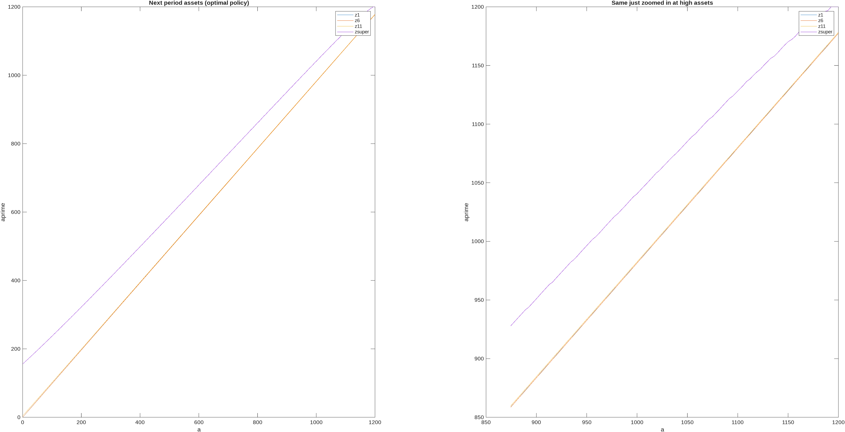
and as you can see it appears essentially linear (the small steps on the right come because there are a few hundred points on labour, they would disappear as you increased the number of points on labour). There are some theory results that tell us that next period assets becomes asymptotically linear in this period assets, e.g., Benhabib, Bisin, and Zhu (2015) show that next period assets (optimal policy) function becomes linear as wealth approaches infinity in a model with capital income risk and liquidity constraints [note: they show for consumption, but next period assets is just resources minus consumption, so applies equally for next period assets]. Ma and Toda (2020) generalize to include capital income; Carroll & Kimball (1996) was an earlier step on this path. Super-star earnings fall within the setups covered by these results.
The next key to the math are results that say that if you have stochastic earnings y_t, and assets accumulate as,
a_{t+1}=\phi a_t + y_t
where \phi is a constant [e.g., as we would get from a linear next period asset function, times a constant rate of return r] then you won’t get fatter tails in the asymptotic distribution of a than you had in y.
There are then further results for processes like
a_{t+1}=\psi_t a_t + y_t
where \psi_t is stochastic. This is called a Kesten process, and there are ‘multiplicative shocks’ \psi_t, alongside the ‘additive shocks’ y_t. These can generate fat tails of the wealth distribution, and, e.g., Nirei & Aoki (2016) show this arises in models with ‘business productivity risks’, but could also arise from things like human capital.
The nail in the coffin was hammered in by Stachurski & Toda (2019). They show that standard Bewley-Imrohoroglu-Huggett-Aiyagari models, without multiplicative shocks, cannot generate a wealth distribution with fatter tails than the earnings distribution.
The reason that entrepreneurial-choice models, among others, escape from this is that the heterogeneous returns to wealth are stochastic and multiplicative, so they look like our \psi_t and we get a Kesten process.
Code that creates the BM2022 graphs shown above. Used Params from the initial stationary eqm and had n_d=301 and n_a=1000,
%% Plot the next period assets
[V,Policy]=ValueFnIter_Case1(n_d,n_a,n_z,d_grid,a_grid,z_grid,pi_z,ReturnFn,Params,DiscountFactorParamNames,[],vfoptions);
PolicyVals=PolicyInd2Val_Case1(Policy,n_d,n_a,n_z,d_grid,a_grid,vfoptions);
figure_c=figure_c+1;
figure(figure_c);
subplot(1,2,1); plot(a_grid,PolicyVals(2,:,1),a_grid,PolicyVals(2,:,6),a_grid,PolicyVals(2,:,11),a_grid,PPolicyVals(2,:,12))
legend('z1','z6','z11','zsuper')
xlabel('a')
ylabel('aprime')
title('Next period assets (optimal policy)')
subplot(1,2,2); plot(a_grid(end-100:end),PolicyVals(2,end-100:end,1),a_grid(end-100:end),PolicyVals(2,end-100:end,6),a_grid(end-100:end),PolicyVals(2,end-100:end,11),a_grid(end-100:end),PolicyVals(2,end-100:end,12))
legend('z1','z6','z11','zsuper')
xlabel('a')
ylabel('aprime')
title('Same just zoomed in at high assets')