If you use ‘AllStats’ one of the outputs is the lorenz curve, and if one of your ‘FnsToEvaluate’ is the ‘assets’ then the lorenz curve of assets is the cumulative shares. Set simoptions.npoints=1000 as the number of points used for the lorenz curve (default is 100).
Then 1-AllStats.assets.LorenzCurve(999) will give you the share of total assets held by the top 0.1%;
2 Likes
Based on the replication of Huggett (1996), I tried…
The ‘LorenzCurve’ command no longer exists. I need to go clean up the Huggett (1996) codes. [I don’t maintain replications, only examples, so the replications can end up outdated. That was before ‘AllStats’ was created, there used to be two or three commands, but it became clear that one command that just gives heaps of model output was much easier to use.]
2 Likes
Thanks. Using your command I got that the share of wealth in top 1% is about 9%, but the authors report 34%. This could be that the grid for assets is too narrow? From @aledinola post, I set maxa=1000 and the inequality results improve: share of top 1% is 18% and gini wealth is 0.8. But this is still not in line with the tables in the paper
1 Like
@javier_fernan I think maxa=1000 is not enough, I used maxa=1200 and maxl=1.5. Actually the policy a'(a,z_{nz}) still hits the upper bound of the asset grid at the very end…
Here are the results of my replication in general equilibrium: see first part of the file for information regarding number of grid points etc., second part for model moments and inequality statistics such as Gini coefficients, shares, etc. The column BM 2022 shows the original model moments in Boar and Midrigan (JME 2022).
NUMERICAL PARAMETERS
------------------------------------------------------------
Hours grid points                       101
Asset grid points                       501
Ability states                           12
Max assets                           1200.0
gridinterplayer                           1
ngridinterp                              30

GENERAL EQUILIBRIUM PARAMETERS AND CONDITIONS
------------------------------------------------------------
r                                  0.022169
iota                               0.334251
B                                  2.000691
G                                  0.144621
capitalmarket                      0.000029
iotacalib                         -0.000087
govdebtcalib                      -0.000116
govbudget                         -0.000054

AGGREGATE MOMENTS
------------------------------------------------------------
Capital                              8.1180
Labor                                0.9930
Hours worked                         0.7589
Output                               2.0005
Capital-to-output                    4.0581
Gov. spending-to-output              0.0723
Walras residual                    0.000014

Moment                              BM 2022   VFIToolkit
------------------------------------------------------------
WEALTH DISTRIBUTION
------------------------------------------------------------
Wealth / Income                      6.6000       6.4958
Gini (Wealth)                        0.8600       0.8165
Top 0.1%% Wealth Share               0.2200       0.0574
Top 1%% Wealth Share                 0.3400       0.1926
Top 5%% Wealth Share                 0.5900       0.4761
Top 10%% Wealth Share                0.7500       0.6644
Bottom 75%% Wealth Share             0.0600       0.0901
Bottom 50%% Wealth Share             0.0000       0.0032
Bottom 25%% Wealth Share             0.0000       0.0000

INCOME DISTRIBUTION
------------------------------------------------------------
Gini (Income)                        0.6500       0.6347
Top 0.1%% Income Share               0.1400       0.1128
Top 1%% Income Share                 0.2200       0.1953
Top 5%% Income Share                 0.4000       0.3733
Top 10%% Income Share                0.5100       0.4939
Bottom 75%% Income Share             0.2700       0.2798
Bottom 50%% Income Share             0.0800       0.1051
Bottom 25%% Income Share             0.0200       0.0268
As you can see, the toolkit does a good job in replicating the income inequality moments but misses the high concentration of wealth at the top.
Here is my code to compute the moments:
FnsToEvaluate2.income  = @(h,aprime,a,z,r,delta,alpha) f_income(h,aprime,a,z,r,delta,alpha);

function pretax_income = f_income(h,aprime,a,z,r,delta,alpha)
% f_income computes Pre-tax income

w = f_prices(r,alpha,delta);

pretax_income = w*h*z+r*a;

end %end function

%% ------------------------------------------------------------------------
% Construct model moments
% -------------------------------------------------------------------------
wealth_to_income = AllStats.A.Mean / AllStats.income.Mean;
gini_wealth      = AllStats.A.Gini;
gini_income      = AllStats.income.Gini;

% Wealth shares
wealth_top01 = 1 - AllStats.A.LorenzCurve(999);
wealth_top1  = 1 - AllStats.A.LorenzCurve(990);
wealth_top5  = 1 - AllStats.A.LorenzCurve(950);
wealth_top10 = 1 - AllStats.A.LorenzCurve(900);
wealth_bot75 =     AllStats.A.LorenzCurve(750);
wealth_bot50 =     AllStats.A.LorenzCurve(500);
wealth_bot25 =     AllStats.A.LorenzCurve(250);

% Income shares
income_top01 = 1 - AllStats.income.LorenzCurve(999);
income_top1  = 1 - AllStats.income.LorenzCurve(990);
income_top5  = 1 - AllStats.income.LorenzCurve(950);
income_top10 = 1 - AllStats.income.LorenzCurve(900);
income_bot75 =     AllStats.income.LorenzCurve(750);
income_bot50 =     AllStats.income.LorenzCurve(500);
income_bot25 =     AllStats.income.LorenzCurve(250);
1 Like
Thanks @aledinola My results for the interest rate and other parameters are different from yours. I realized now that I haven’t corrected FnsToEvaluate.TaxRevenue, maybe it’s that.
1 Like
With respect to @robertdkirkby code, I suggest these changes:
(1) Include consumption taxes in the function that computes total tax revenues
(2) Increase the upper bound for d_grid to 1.5
(3) Increase upper bound for a_grid to (at least) 1200
(4) Add the calculation of some inequality moments for income and wealth, see code posted above
(1) and (3) are the most important ones.
1 Like
I have done all your suggestions and now I can replicate your results. Top wealth shares and top 0.1% income share are still off the mark, by quite a lot. Wonder if there is an issue with the replication or with the paper itself.
Pushed updated version of BM2022 code that does (1)-(4). Thanks for the nice clean list!
I expect that the numbers in the paper for wealth inequality contain non-negligible numerical error. This kind of model should fail at getting the wealth distribution to have a fatter tail than the income distribution, so what the toolkit code gives seems much more likely to be correct than the paper.
3 Likes
In my code I tried to improve the general equilibrium algorithm by choosing fminalgo=5 but in that case it does not converge. In principle it should be faster than fminalgo=1 which relies on a ‘blind’ minimization routine.
@robertdkirkby I wonder if you tried that too
I haven’t tried it as I am too lazy to write out update rules ![]() (I only write them for transition paths because it is not yet possible to skip doing so, hopefully sometime soon I get around to making it so they are not needed there either) That said, they can be very fast when you set them up right. If you think it might be an issue with toolkit though, then let me know and I will go try do it
(I only write them for transition paths because it is not yet possible to skip doing so, hopefully sometime soon I get around to making it so they are not needed there either) That said, they can be very fast when you set them up right. If you think it might be an issue with toolkit though, then let me know and I will go try do it ![]()
Nowadays when I want faster I always use ‘lsqnonlin’ which is fminalgo=8. Is decently faster than ‘fminsearch’ (default fminalgo=1) and requires zero extra setup.
1 Like
My understanding was that adding a super-star shock to an aiyagari model would allow the model to get a very high concentration of wealth at the top
As far as accuracy is concerned, it would be interesting to compute the residuals of the Euler equation and the first order condition for labor.
1 Like
Euler Equation Residuals are invalid for this model. I figured this deserved a post of it’s own:
[is a minor reworking of two big footnotes about what is wrong with EERs from my Quantitative Macroeconomics replication paper, but I added some stuff about how we can know if we have the true solution]
2 Likes
Great point. What about the residual of the labor foc? It holds as equality.
Hmm, good point. Following is me freewheeling.
You could still evaluate the residual of the labor FOC. Satisfying the labor FOC is a necessary condition for the model solution to be internally consistent.
I’m not sure you could say anything from the labor FOC about more generally whether the policy function is accurate, and whether model statistics (say the Gini of Income or Gini of Wealth) are accurate.
So big residuals for the labor FOC will tell you the solution accuracy is not great, but small residuals cannot tell you that the solution more generally is accurate.
I guess one weakness is the same kind of bias you get with EERs in the sense if you put lot’s of points on labor supply (but few on assets and shocks) you can get the residuals of the labor FOC very small even though the rest of the model is not very accurate.
[This is all hand waving stuff, I cannot think of any theory about small errors in just one model equation telling you about possible errors in the other model equations. I’d be interested to know if there is any.]
In any paper you are going to report a bunch of model statistics, maybe the Gini of Wealth, or the age conditional means of income, or even the CEV for welfare. Really what you care about is the accuracy of the model stats you are going to report (if you are only reporting the mean of wealth, you don’t really care if the wealth share of the top 0.1% is being accurately solved as long as the mean is accurate). So the question is whether errors in this FOC (which you don’t directly care about) will cause non-negligible numerical errors in the model stats you do care about and plan to report.
2 Likes
Unrelated: I think there is still a typo in BoarMidrigan2022_ReturnFn.m, should divide by (1+tau_s) instead of (1-tau_s).
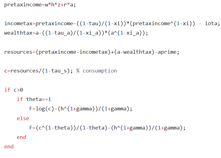
@javier_fernan: As @robertdkirkby has already explained, EER are not a good way of assessing accuracy. Out of curioisty, I have computed the residuals for the labor foc:
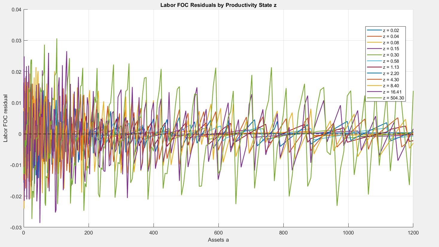
It was quite easy with the help of ChatGPT 5.2 ![]()
Here is the code if you are interested:
function [resid, pol_c] = fun_foc_resid(n_a,n_z,a_grid,z_grid,PolicyValues,P)

wage  = f_prices(P.r,P.alpha,P.delta);

% Gather and reshape policy functions
z_grid      = gather(z_grid);
PolicyValues = gather(PolicyValues);
pol_h       = reshape(PolicyValues(1,:,:), [n_a, n_z]);
pol_aprime  = reshape(PolicyValues(2,:,:), [n_a, n_z]);

% Compute policy function for consumption
% f_consumption(h,aprime,a,z,r,tau_s,tau,xi,tau_a,xi_a,iota,delta,alpha);
pol_c = zeros(n_a,n_z);
for z_c = 1:n_z
    z = z_grid(z_c);
    for a_c = 1:n_a
        h      = pol_h(a_c,z_c);
        aprime = pol_aprime(a_c,z_c);
        a      = a_grid(a_c);

        pol_c(a_c,z_c) = f_consumption( ...
            h, aprime, a, z, ...
            P.r, P.tau_s, P.tau, P.xi, ...
            P.tau_a, P.xi_a, P.iota, P.delta, P.alpha);
    end
end

% Compute residual from labor first order condition
resid = zeros(n_a,n_z);
for z_c = 1:n_z
    z = z_grid(z_c);
    for a_c = 1:n_a
        a = a_grid(a_c);
        c = pol_c(a_c,z_c);
        h = pol_h(a_c,z_c);

        LHS      = h^P.gamma;
        marg_tax = 1-(1-P.tau)*(P.r*a+wage*z*h)^(-P.xi);
        RHS      = ((1-marg_tax)/(1+P.tau_s))*c^(-P.theta)*wage*z;

        resid(a_c,z_c) = LHS-RHS;

    end
end

resid = gather(resid);
pol_c = gather(pol_c);

end % end function
I think the function could be simplified by using a toolkit command to compute the policy function of consumption. @robertdkirkby Do you remember how to do this?
The policy function for consumption can be computed by creating a FnsToEvaluate.Consumption and then just doing ValuesOnGrid. The resulting ValuesOnGrid.Consumption is the policy function for consumption.
1 Like
This is correct. But incomplete.
‘Super-star’ earnings (one value on the earnings grid that is much larger than the rest, but also very low probability) does give much higher earnings and wealth than a model without (say a model with AR(1) earnings). This was the breakthrough of Castañeda, Díaz‐Giménez & Ríos‐Rull (2003) which was the first to show how you can get plausible earnings and wealth inequality in a Bewley-Imrohoroglu-Hugget-Aiyagari model, which they did by calibrating the values and transition probabilities of a markov, with the calibration resulting in the model having ‘super-star’ earnings.
But since then we have learned more and the bar has been raised on what it means to get realistic levels of wealth inequality. In particular, we nowadays understand that just using ‘super-star’ earnings will result in a model that falls into the class of models which fail to get a fatter tail of the wealth distribution than for the earnings distribution. The empirical distribution of wealth always (every year and every country you care to look at) has a fatter tail than the empirical distribution of earnings.
Currently the most widely used trick in the literature to get models that can both generate plausible earnings and wealth inequality and can get a fatter tail of the wealth distribution than of the earnings distribution are entrepreneurial-choice models. The key mechanism here is the heterogeneous returns to assets, which means these models escape the class of models that cannot have fatter tails of the wealth distribution than of the earnings distribution.
Note that this is a bit disguised when you look at super-star earnings model as they often have a fairly small finite number of values in the earnings distribution, but a whole continuum of values in the wealth distribution.
Of course there is no reason why your model needs to go beyond the ‘plausible’ earnings and wealth distribution that ‘super-star’ earnings delivers, and get the more realistic fatter tails of the wealth distribution that entrepreneurial-choice models (among others) can deliver, unless the difference is something that is relevant to the economic question you are asking the model.
2 Likes
What is the intuition for why a standard Aiyagari model, even with super-star earnings, cannot generate a fatter tail of the wealth distribution than of the earnings distribution?
First, notice that for higher levels of assets, next period assets is a linear function of this period assets. Here is a graph of this from the Boar & Midrigan (2022) model,
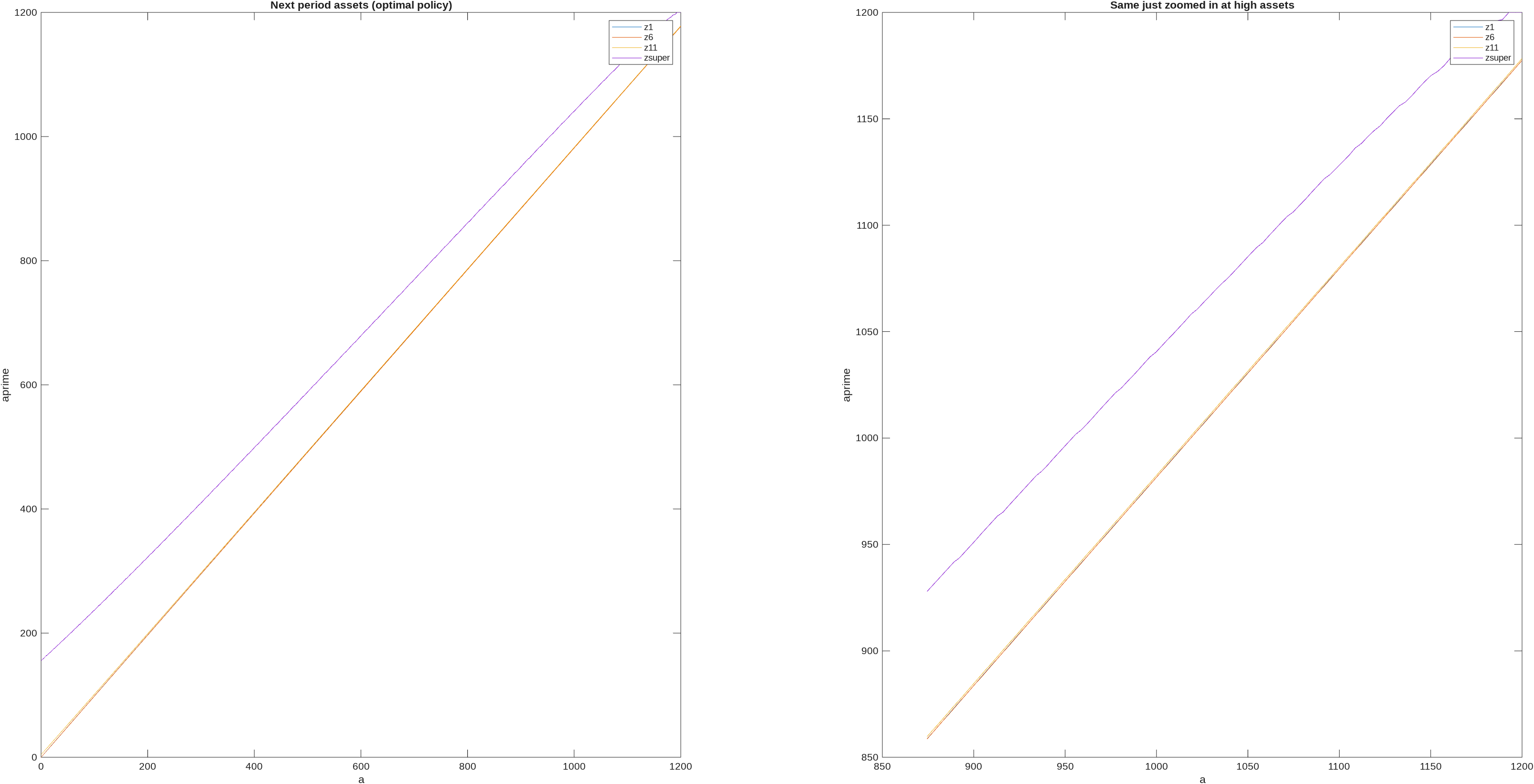
and as you can see it appears essentially linear (the small steps on the right come because there are a few hundred points on labour, they would disappear as you increased the number of points on labour). There are some theory results that tell us that next period assets becomes asymptotically linear in this period assets, e.g., Benhabib, Bisin, and Zhu (2015) show that next period assets (optimal policy) function becomes linear as wealth approaches infinity in a model with capital income risk and liquidity constraints [note: they show for consumption, but next period assets is just resources minus consumption, so applies equally for next period assets]. Ma and Toda (2020) generalize to include capital income; Carroll & Kimball (1996) was an earlier step on this path. Super-star earnings fall within the setups covered by these results.
The next key to the math are results that say that if you have stochastic earnings y_t, and assets accumulate as,
a_{t+1}=\phi a_t + y_t
where \phi is a constant [e.g., as we would get from a linear next period asset function, times a constant rate of return r] then you won’t get fatter tails in the asymptotic distribution of a than you had in y.
There are then further results for processes like
a_{t+1}=\psi_t a_t + y_t
where \psi_t is stochastic. This is called a Kesten process, and there are ‘multiplicative shocks’ \psi_t, alongside the ‘additive shocks’ y_t. These can generate fat tails of the wealth distribution, and, e.g., Nirei & Aoki (2016) show this arises in models with ‘business productivity risks’, but could also arise from things like human capital.
The nail in the coffin was hammered in by Stachurski & Toda (2019). They show that standard Bewley-Imrohoroglu-Huggett-Aiyagari models, without multiplicative shocks, cannot generate a wealth distribution with fatter tails than the earnings distribution.
The reason that entrepreneurial-choice models, among others, escape from this is that the heterogeneous returns to wealth are stochastic and multiplicative, so they look like our \psi_t and we get a Kesten process.
Code that creates the BM2022 graphs shown above. Used Params from the initial stationary eqm and had n_d=301 and n_a=1000,
%% Plot the next period assets
[V,Policy]=ValueFnIter_Case1(n_d,n_a,n_z,d_grid,a_grid,z_grid,pi_z,ReturnFn,Params,DiscountFactorParamNames,[],vfoptions);
PolicyVals=PolicyInd2Val_Case1(Policy,n_d,n_a,n_z,d_grid,a_grid,vfoptions);
figure_c=figure_c+1;
figure(figure_c);
subplot(1,2,1); plot(a_grid,PolicyVals(2,:,1),a_grid,PolicyVals(2,:,6),a_grid,PolicyVals(2,:,11),a_grid,PPolicyVals(2,:,12))
legend('z1','z6','z11','zsuper')
xlabel('a')
ylabel('aprime')
title('Next period assets (optimal policy)')
subplot(1,2,2); plot(a_grid(end-100:end),PolicyVals(2,end-100:end,1),a_grid(end-100:end),PolicyVals(2,end-100:end,6),a_grid(end-100:end),PolicyVals(2,end-100:end,11),a_grid(end-100:end),PolicyVals(2,end-100:end,12))
legend('z1','z6','z11','zsuper')
xlabel('a')
ylabel('aprime')
title('Same just zoomed in at high assets')
3 Likes