Replication of Boar and Midrigan (2022)

You are right. I had missed this. Nice spot, thanks!

I have just fixed and updated the Boar & Midrigan (2022) codes. Uses intermediateEqns to handle K=A-B. I implemented intermediateEqns for the transition path as part of fixing this example, so is nice and easy for user now. Even though intermediateEqns adds zero extra functionality I do like how much easier it makes code to read (I think it makes typo mistakes in setting up the model much less likely; plus seeing the intermediates during the iterations makes diagnosing what is going on easier too).

I also turned the grids up larger, I suspect this example is now more accurate than the original. And I added using the new ‘AllStats’ for ‘TPath’ which makes it super easy to get, in this example, the Gini of wealth over the transition path.

Because this is the kind of model where EGM (endogenous grid method) works the toolkit is obviously not as fast as custom code. But on the plus side it is very easy to solve.

PS. Not sure how I missed it, I literally have a paper in progress where we do this exact K=A-B trick in our general eqm eqns. Oh well, fixed now so all good.

1 Like

Nice! I was wondering if the code for BM 2022 is available somewhere. I did not find it after a quick google search. I did find the code to replicate the model with entrepreneurs (published in AER:Insights).

In your repo you write that BM 2022 use Rouwenhorst. May I ask where they state this? Related to the discretization of labor ability, did you choose nz=11 (12 with the super-star) shock based on something they write in the paper?

Online Appendix B: “We solve the model by discretizing the distribution of labor market ability e using a Rouwenhorst method with 11 points. We approximate agents’ value and consumption functions in the wealth space with 501 linear splines.”
They do some brief discussion of algorithms. They use something based on the Euler eqns (not sure why they don’t use EGM, surely it would be better?). Unfortunately vague on what they do with labor supply.

I agree. Pretty sure the code is not public. Unfortunately the JME editors are a bunch of troglodytes who don’t require code to be published :face_with_steam_from_nose:, not like the enlightened folk at AER:Insights :wink:

1 Like

Thanks! Regarding the algorithm, I had a look at their AER code and they use a modified value function iteration with golden section search and linear interpolation.

(1) The choice variable is labor supply h.

(2) Given h, they obtain consumption from the intratemporal first order condition wrt labor supply. Note that consumption can be solved analytically as a function of h and of the state variables, even with nonlinear tax functions. Here having a differentiable tax function like HSV is helpful.

(3) Given h and c, obtain a' from the budget constrain. If a'<0, assign a large penalty proportional to abs(a’), but not infinity.

(4) Since the a' obtained in the previous step is unlikely to be on the grid, linearly interpolate the future value function.

In the appendix they discuss a method based on Euler equations and envelope condition which requires rootfinding (so, not EGM). But in the AER code they seem to use the algorithm I described above.

I agree that EGM should be faster than both Euler equation with rootfinding and value function iteration, but I am not sure EGM is feasible in the model with entrepreneurs.

I tried their value function iteration and it is fast, it takes 0.5 seconds on my laptop. The trick is that they use a vectorized version of the golden section algorithm, from the toolbox of Miranda and Fackler. I show below the vectorized golden search function.

GOLDENX Computes local maximum of univariate function on interval via Golden Search
 
%   Vectorized version of Golden
 
% USAGE
 
%   [x,fval] = goldenx(f,a,b,P1,P2,...);
 
% INPUTS
 
%   f         : name of function of form fval=f(x)
 
%   a,b       : left, right endpoints of interval
 
%   P1,P2,... : optional additional arguments for f
 
% OUTPUTS
 
%   x       : local maximum of f
 
%   fval    : function value estimate
 
%
 
% USER OPTIONS (SET WITH OPSET)
 
%   tol     : convergence tolerance
 
 
% Copyright (c) 1997-2002, Paul L. Fackler & Mario J. Miranda
 
% paul_fackler@ncsu.edu, miranda.4@osu.edu
 
 
function [x1,f1] = goldenx(f,a,b,varargin)
 
 
tol = optget('goldenx','tol',sqrt(eps));
 
 
alpha1 = (3-sqrt(5))/2;
 
alpha2 = 1-alpha1;
 
d  = b-a;
 
x1 = a+alpha1*d;
 
x2 = a+alpha2*d;
 
s  = ones(size(x1));
 
f1 = feval(f,x1,varargin{:});
 
f2 = feval(f,x2,varargin{:});
 
 
d = alpha1*alpha2*d;
 
while any(d>tol)
 
  i = f2>f1;
 
  x1(i) = x2(i);
 
  f1(i) = f2(i);
 
  d = d*alpha2;
 
  x2 = x1+s.*(i-(~i)).*d;
 
  s = sign(x2-x1);
 
  f2 = feval(f,x2,varargin{:});
 
end
 
 
% Return the larger of the two
 
i = f2>f1; x1(i) = x2(i);  f1(i) = f2(i);
 

Yeah, EGM wouldn’t work (or at least not remotely easy) for BM2023 because of the permanent-entrepreneurs. It would work for BM2022. I take it from your description that the BM2023 then involves a grid on labor supply h.

BM2023 define grids on assets, worker ability and entrepreneurial ability. Labor supply is chosen by the golden section search algorithm in a bounded interval, so there is no grid over labor supply.

Talking about labor supply, I think it is not correct to impose the upper bound for labor supply at 1.

Given the preferences used,

\log(c) - \frac{h^{1+\gamma}}{1+\gamma}

the optimal hours of work can be larger than one. This is similar to Bruggeman (2021) where she sets the upper bound for the hours grid equal to 1.6 (see variables minl and maxl in her Fortran code). Note that neither Boar and Midrigan (2022) nor Bruggeman (2021) ever impose the constraint h \leq 1 in their respective papers.

Are you suggesting to solve for the stationary equilibrium 100 times? I am trying to understand how to compute optimal tax rates in this kind of models and I am a bit lost

BTW, Thanks for the code, it’s great

I suspect you are right about not imposing h<=1. Without their code we cannot see if they have a max h. I guess I just have to solve a few times to find a suitable max h.

1 Like

Start from the definition: the optimal tax rates are the tax rates that maximize welfare. So mathematically,
\tau*=arg\max_{\tau} Welfare(\tau)
where \tau is the tax rate(s) [in BM2022 this is four taxes, but I will write it as a vector to keep notation simpler].

Welfare(\tau) is the social welfare function, evaluated based on solving the model with tax rate \tau. So to evaluate some value of \tau we need to (i) solve the model, and (ii) calculate the social welfare function.

There are two possible exercises here. In some papers, like Conesa, Kitao & Krueger (2009) step (i) solving the model means computing the stationary eqm, and then step (ii) is the social welfare function evaluated in terms of the stationary eqm. In BM2022 step (i) solving the model means computing the final stationary eqm and the transition path to this, and then step (ii) is the social welfare function evaluated in terms of the transition path.

That covers how to calculate Welfare(\tau) for a given \tau. From a computational perspective we would want to set up a function that takes in \tau, and then (i) solves the model, and (ii) calculates social welfare, and then outputs the social welfare Welfare(\tau).

The other part is how to solve the maximization problem arg\max_{\tau} Welfare(\tau). There are lots of ways to compute an optimization problem.

We could just put a grid on \tau and try to find the ‘best’ \tau on this grid; we could use our function that takes input \tau and gives output Welfare(\tau) and just evaluate this on the grid (do a loop over the grid on \tau, and evaluate our function to get Welfare(\tau) for each point on the grid, then pick the maximum of them).

We could ‘fully’ solve the maximization problem by using some algorithm/command for optimization. For example, we could pass it to the Matlab commands fminsearch() or lsqnonlin(), or to other commands like CMA-ES (all three of these are things VFI Toolkit uses for optimization when solving things like stationary eqm, or calibrating a model). Note that most optimization routines are for minimization, so we would need to minimize -Welfare(\tau) (mimimizing negative x is maximizing x). In these examples we are passing our function that takes input \tau and gives output Welfare(\tau) as the function to be maximized (or more accurately minus this function to be minimized).

The approach taken by BM2022 is to first do the ‘grid’ exercise, and then use the solution to this as an initial guess for the ‘full’ optimization exercise. The grid is easier, but not as accurate, and getting a good initial guess makes the optimization both much faster and much more robust.

All of what I have described is is ‘nested optimization’ (we first do an inner ‘find model eqm’ optimization, and then an outer ‘find max welfare’ optimization). In principle there is also the alternative of ‘joint optimization’ but I won’t go into that here as for this exercise it is not trivial how to setup the relative weights, and I don’t see people using it for optimal tax exercises although in principle if it works it would be faster than the nested optimization.

1 Like

In the AER:Insights, they set the interval for golden search as

h \in [\bar{h}, \bar{h} + 5]

where \bar{h} is the smallest h that ensures a'=0 (note that such hbar depends on current assets a and on workers’ ability e). I don’t think the upper bound is ever binding of course, you just have to define an interval for the routine solve_golden. The lower bound might be binding instead. Here is the relevant part of the authors’ code:

 
function [v, h] = bellman(hbar, varargin)


hmin      = hbar;                                                          
 
hmax      = hbar + 5;                                   % bounds on hours
 
 
h         = solve_golden('valfunc', hmin, hmax, varargin{:}); 
 
 
v         = valfunc(h, varargin{:}); 
 
 
vbar      = valfunc(hbar, varargin{:}); 
 
 
h         = h.*(v > vbar) + hbar.*(v <= vbar); 
 
 
v         = v.*(v > vbar) + vbar.*(v <= vbar); 


I set the max for h to 2. Solved the initial and final stationary eqm, and no-one chooses more than 1.2. So I have updated the BM2022 codes with max for h_grid of 1.3.

The code to see the cdf of h was,

%% Find suitable max of the labor supply
FnsToEvaluate3.H=@(h,aprime,a,z) h;
ValuesOnGrid=EvalFnOnAgentDist_ValuesOnGrid_Case1(Policy_init,FnsToEvaluate3,Params_init,[],n_d,n_a,n_z,d_grid,a_grid,z_grid,simoptions);
[h_vals,~,hind]=unique(ValuesOnGrid.H);
h_pdf=accumarray(hind,StationaryDist);
h_cdf=cumsum(h_pdf);
ValuesOnGrid2=EvalFnOnAgentDist_ValuesOnGrid_Case1(Policy_final,FnsToEvaluate3,Params,[],n_d,n_a,n_z,d_grid,a_grid,z_grid,simoptions);
[h_vals2,~,hind2]=unique(ValuesOnGrid2.H);
h_pdf2=accumarray(hind2,StationaryDist_final);
h_cdf2=cumsum(h_pdf2);
plot(h_vals,h_cdf,h_vals2,h_cdf2)
legend('initial eqm', 'final eqm')
title('cdf of hours worked in stationary general eqm')

[code does not currently create Params_init, but just put Params_init=Params; shortly after solving the initial stationary eqm so as to keep a copy.]

1 Like

Interesting! One question: Valuesongrid.H is the policy function for hours? Can I just obtain it from Policyind2val?

One question: Valuesongrid.H is the policy function for hours? Can I just obtain it from Policyind2val?

Yes. This is equivalent.

The ValuesOnGrid approach is obviously more flexible as you can use it for any FnsToEvaluate.

Actually, internally the EvalFnOnAgentDist type commands tend to call PolicyInd2Val and then pass the policy values (after permuting them) into the FnsToEvaluate.

1 Like

Dear Robert, thank you for your very clear explanation. I have one remaining question about the paper’s economic rationale: given the absence of return heterogeneity, I am unclear on why wealth taxes are required.

Two comments on your BM2022 example:

Consumption taxes. I think you forgot to include consumption taxes when defining total tax revenues in line 116 of your main scirpt:

FnsToEvaluate.TaxRevenue=@(h,aprime,a,z,r,tau,xi,iota,delta,alpha,tau_a,xi_a) BM2022_IncomeTaxRevenue(h,aprime,a,z,r,tau,xi,iota,delta,alpha) + BM2022_WealthTaxRevenue(h,aprime,a,z,tau_a,xi_a);

In fact, the government collects taxes on personal income, wealth and consumption (the consumption tax rate is \tau_s).

Improve general equilibrium algorithm. If I choose fminalgo=5 (shooting), I set

GEPriceParamNames_pre = {'r','iota','B','G'};

heteroagentoptions.intermediateEqns.K=@(A,B) A-B; % physical capital K: A is asset supply, K and B are asset demand 
heteroagentoptions.intermediateEqns.Y=@(K,L,alpha) (K^(alpha))*(L^(1-alpha)); % output Y

% --- Interest rate equals marginal product of capital (net of depreciation)
GeneralEqmEqns_pre.capitalmarket = @(r,K,L,alpha,delta) r-(alpha*(K/L)^(alpha-1)-delta); 
% --- Calibration target iota/Y 
GeneralEqmEqns_pre.iotacalib     = @(iota,iota_target,Y) iota_target - iota/Y; % get iota to GDP-per-capita ratio correct
% --- Calibration target B/Y 
GeneralEqmEqns_pre.govdebtcalib  = @(Bbar,B,Y) Bbar - B/Y; % Gov Debt-to-GDP ratio of Bbar
% --- Balance the goverment budget
GeneralEqmEqns_pre.govbudget     = @(r,B,G,TaxRevenue) r*B+G-TaxRevenue;

% Option for shooting algo
heteroagentoptions.fminalgo5.howtoupdate={... % a row is: GEcondn, param to adjust, add (if 1), factor
    'capitalmarket','r',0,0.05;... % CapitalMarket GE condition will be positive if r is too big, so subtract
    'iotacalib','iota',1,0.05;... % govbudget GE condition positive if iota is too small, so add
    'govdebtcalib','B',1,0.01;... % govdebtcalib condition positive if B is too small, so add
    'govbudget','G',0,0.01;...    % govbudget condition positive is G is too big, so subtract
     };

Does this make sense to you? Unfortunately, it does not converge: in particular, the condition govbudget goes further and further away from zero after two iterations. I am wondering if I should set 1 instead of 0 for G.

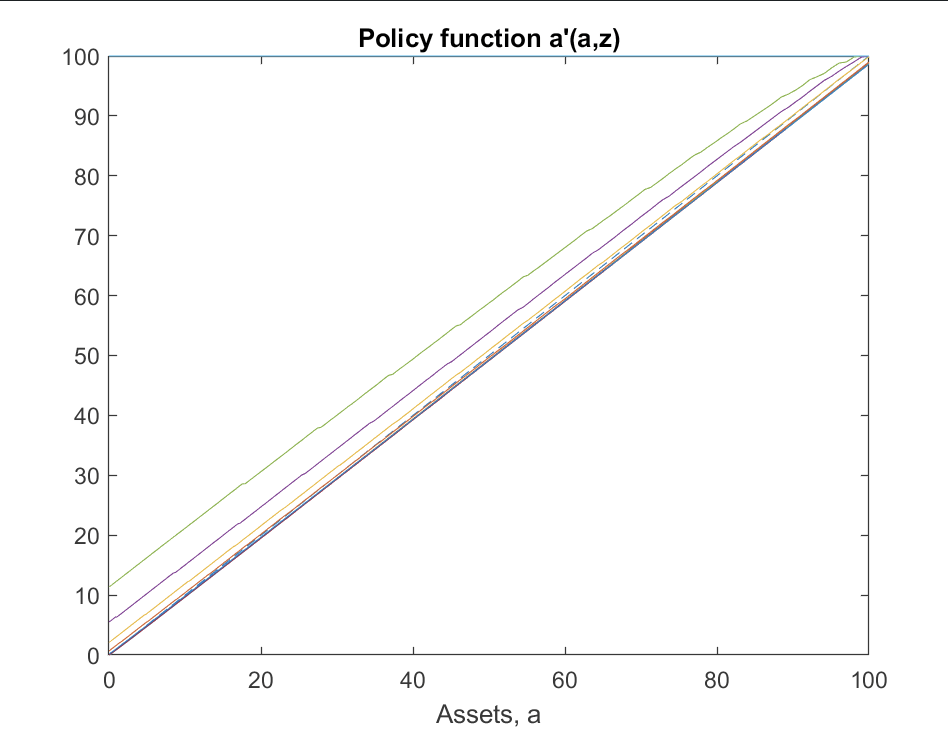
Upper bound for assets
Given the super-star shock, are you sure maxa = 100 is sufficient? If I plot the policy function a'(a,z) for the highest z, is hits the upper bound (see graph below). There are only 0.02% of agents in the super-star state, so maybe it does not transpire well if you only look at the stationary distribution.

2 Likes

BM2022 has rate or return homogeneity, which is to say everyone gets the same rate of return, r, on their assets, a.

In this situation, a capital income tax, \tau_k, levied on capital income, ra, is indistinguishable from a wealth tax, \tau_a, levied on wealth, a. You either pay capital income tax \tau_k r a or you pay wealth tax \tau_a a, but as it clear to raise the same revenues you would need \tau_a=\tau_k r, and so they are doing the exact same thing. [In stationary eqm, as this assumes r is also constant.]

There are models with rate of return heterogeneity, different agents get different r, in which capital income taxes and wealth taxes have different effects. Mostly people use entrepreneurial-choice models for this, although portfolio-choice models also technically achieve this. A key reference is Guvenen, Kambourov, Kuruscu, Ocampo & Chen (2023).

So in BM2022 there is no difference between a wealth and a capital income tax. They happen to choose to have a wealth tax, but it would be no difference to if they used a capital income tax. [This is actually not quite true, because r differs over the transition path.] Note that their other tax is on ‘all’ income —labor income plus capital income— so the two taxes they use are distinct, albeit with an overlapping tax base. BM2022 Section 4.6 does do separate taxation of labor income and capital income, but seems to be done just for ‘comparison to literature’ and doesn’t talk about how capital income tax differs (or does not differ) from wealth tax.

Plausibly, BM2022 deliberately use a wealth tax rather than capital income tax precisely due to the difference over the transition, where changing r means the capital income tax ‘varies’ more than the wealth tax. But I don’t think they discuss this anywhere, so more likely is just coincidence/luck; they just say “a non-zero wealth tax simply allows for differential taxation of labor and capital income”.

1 Like

Thanks for your very detailed answer. I will read Guvenen et al. paper that you referenced.

Thanks for your post, @aledinola. My understanding from the chart you uploaded is that agents in the super-star state always choose a’=100. Is this why you suggest increasing the upper bound of the assets grid? I checked the gini of assets AllStats_init.A.Gini and it is equal to 0.7 which is less than 0.86 reported by the authors. I would like to check the shares of wealth owned by verious percentiles of the wealth distribution: I know that in these models it is important to replicate the high concentration of wealth at the top. The authors report that in the model the wealth share of the top 0.1% is equal to 22%. How can I compute the share with the toolkit?

Thanks for your help.

1 Like

Based on the replication of Huggett (1996), I tried

AllLorenzCurves=EvalFnOnAgentDist_LorenzCurve_FHorz_Case1(StationaryDist, Policy, FnsToEvaluate, Params, [], 0, n_a, n_z,N_j, 0, a_grid, z_grid);
TopWealthShares=100*(1-AllLorenzCurves.K([80,95,99],1));

but I get an error