Thanks for the answer! Totally makes sense.
I didn’t notice the number of iterations is much higher with interpolation, I’ll have a look
Thanks for the answer! Totally makes sense.
I didn’t notice the number of iterations is much higher with interpolation, I’ll have a look
Again using the Pijoan-Mas example, I tried to do some calibration using the general equilibrium function.
If I simply want to find the general equilibrium, I would have to
Guess the aggregate capital-to-labor ratio \frac{K}{L} .
Find the implied interest rate and wage as:
r = (1 - \theta) \left( \frac{K}{L} \right)^{-\theta} - \delta
w = \theta \left( \frac{K}{L} \right)^{1 - \theta}
Solve the household’s problem given prices (r, w) , and obtain the policy functions:
Compute the stationary distribution ( \mu(a, z) ).
Compute aggregate capital and labor:
\hat{K} = \int a \, d\mu(a, z), \quad
\hat{L} = \int z \, g_h(a, z) \, d\mu(a, z)
Iterate until:
\left| \frac{K}{L} - \frac{\hat{K}}{\hat{L}} \right| < \varepsilon
But what if I also want to calibrate \beta so that in equilibrium the capital-to-output ratio is equal to, say, 3?
Thanks to the Toolkit, it is very easy. Simply add the calibration target as an additional GE condition:
GeneralEqmEqns.CapitalMarket = @(K_to_L,K,L) K_to_L-K/L;
% More GE conditions as targets
GeneralEqmEqns.target_beta = @(K,L,theta) K/(K^(1-theta)*L^theta) - 3.0;
The code above tells the toolkit that we want to clear the capital market by finding the appropriate K/L ratio but also that we want K/Y to be as close to 3.0 as possible.
Since we have two GE conditions, we need two parameters. These are K/L and beta:
GEPriceParamNames = {'K_to_L','beta'};
heteroagentoptions.constrain0to1 = {'beta'};
Note that we want to constrain \beta to be in (0,1) and we do that with the option constrain0to1.
Bug alert!
All good so far. I ran the code and it solves the modified GE problem (of course I started with a great initial condition, from the paper). As a last step, I update the parameters K/L and \beta to the values found by the GE algorithm as follows
Params.K_to_L = 5.56527812096859;
Params.beta   = 0.945362091782898;
and run again with heteroagentoptions.maxiter = 0. Unfortunately I get wrong results:
Current GE prices:
	K_to_L:   5.5653
	beta:   0.7202
Current aggregate variables:
	K:   0.0000
	L:   0.4396
	H:   0.3948
Current GeneralEqmEqns:
	CapitalMarket:   5.5653
	target_beta:  -2.9998
GeneralEqmCondn:
    CapitalMarket: 5.56527584636577
      target_beta: -2.99975542077336
I know they are wrong since with these values of K/L and beta, the GE conditions were close to zero.
The problem now is that beta is not equal to the value I gave but to something else ![]()
My guess is that there is something wrong with the transformation to restrict beta in (0,1). Like it is not converted back if maxiter=0?
Regarding the comparison of interp vs no interp.
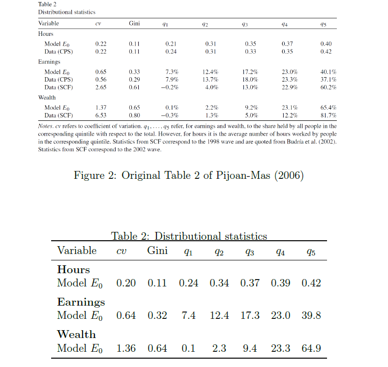
I didn’t notice any meaningful difference in the model moments between the two methods. I managed to replicate the first two tables of Pijoan-Mas (2003) relatively easily.
This shows for example the original Table 2 in the paper vs Table 2 in my replication exercise:
I guess this model is smooth (no non-convexities, fixed cost, etc) so using either method does not matter much.
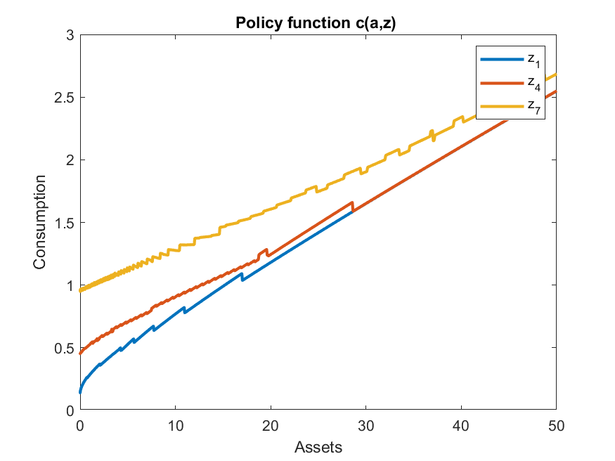
The policy function for consumption, however, looks very different with interpolation compared to pure discretization. With pure discretization, even with 1000 points for assets and 100 points for hours, it looks quite zig-zag:
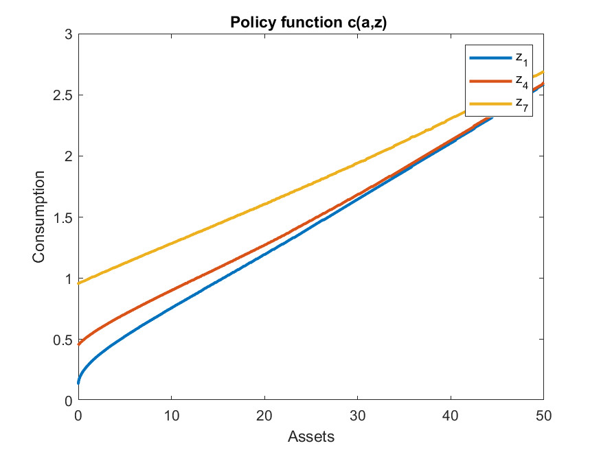
With interpolation on, the same policy function looks instead
Getting right the policy for consumption might be important for welfare
Question
One of the distributional statistics reported in Table 2 of Pijoan-Mas is the average hours by quintile of hours (see also note to the table). I computed these numbers “by hand” in the function fun_hours_means. Is there a way to do this computation in the toolkit?
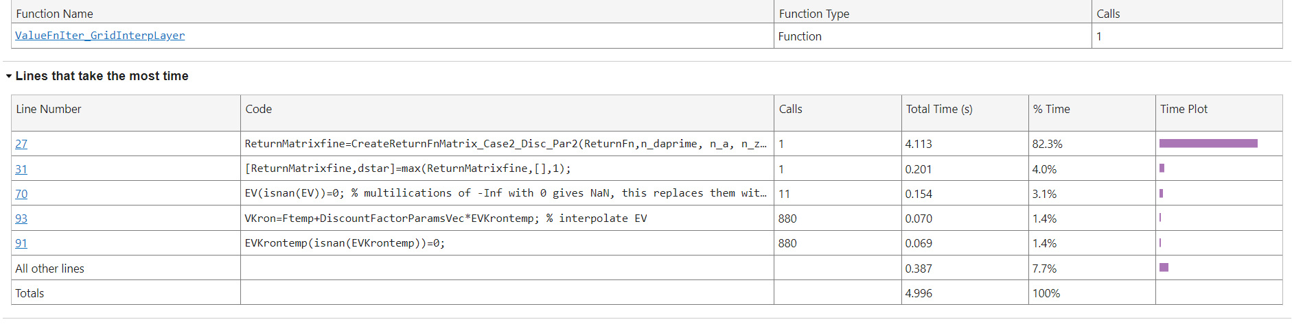
Regarding the slow performance of the code with interpolation. I ran the VFI with profiler and most of the time is spent in creating the return matrix.
The file below shows the lines of ValueFnIter_Refine_preGI_raw that takes the most time. The culprit is clearly the call to CreateReturnFnMatrix_Case2_Disc_Par2 on line 27 and the creation of ReturnMatrixfine which is a huge array. Overall the two iterations parts are fast and the second takes 16 iterations (which is in line with my experience with Howard).
Fixed the use of constraints when heteroagentoptions.maxiter=0.
Yes.
Advanced but flexible way: Run AllStats twice. First run set simoptions.nquantiles=5 so you get the quintile cut-offs for hours. Then set up five simoptions.conditionalrestrictions.q1 (for q1 to q5) which evaluate to zero if hours is between the cut-offs for the hours quintile. Then run AllStats again, and you will get earnings stats conditional on being in that quintile. (Note: if you used, e.g., earnings in first step and then hours in second step this approach would give you mean hours conditional on earnings quintile. This approach also gives things like the variance of hours conditional on earnings quintile.)
Easy way, but won’t generalize beyond this example: Actually in this case it is even easier than that, because you want the mean for the quintile. So all you need is to set simoptions.nquantiles=5 and then it will report the quantile means for you. (The only things reported in this way are the quantile means and the quantile cut-offs.)
I have updated my example based on Pijoan-Mas. I have included the internal calibration of the preference parameters \beta, \lambda, \sigma and \nu as part of the general equilibrium calculation.
u(c,\ell) = \frac{c^{1-\sigma}}{1-\sigma} + \lambda \frac{(1-\ell)^{1-\nu}}{1-\nu}
| Parameter | Description | Calibration Target |
|---|---|---|
| \beta | Discount factor | Capital-output ratio |
| \lambda | Weight of leisure | Average hours |
| \sigma | Risk aversion | Corr(h,z) |
| \nu | Inverse of leisure elasticity | cv(h) |
I did this thanks to the new feature CustomStats. Indeed, the calibration targets for \sigma and \nu are the correlation between hours and productivity, corr(h,z) and the coefficient of variation of hours, cv(h). Since these targets are not means or aggregate variables, they cannot be computed as part of the standard general equilibrium routine.
It was a useful exercise to learn how to find general equilibrium AND calibrate internally a bunch of parameters to hit some targets, using the VFI toolkit. I hope some users find this helpful. @robertdkirkby feel free to include my example among the Heterog Agents Examples of the toolkit, if you think might be useful. There is already Aiyagari, but this based on Pijoan-Mas (2003) has a d variable, so may be useful to test/debug.
Here is the link to the repo:
My code for the function that computes “customized statistics”:
function custom_stats = fun_custom_stats(V,Policy,StationaryDist,Params,FnsToEvaluate,n_d,n_a,n_z,d_grid,a_grid,z_gridvals,pi_z,heteroagentoptions,vfoptions,simoptions)
% CustomStats=Aiyagari1994_CustomModelStats(V,Policy,StationaryDist,Parameters,FnsToEvaluate,n_d,n_a,n_z,d_grid,a_grid,z_gridvals,pi_z,heteroagentoptions,vfoptions,simoptions)
% % CustomStats: output a structure with custom model stats by fields with the names you want
% % The inputs to CustomModelStats() are fixed and not something the user can
% % change. They differ based on InfHorz of FHorz, and differ if using PType.
% % Note: Most of them are familiar, only thing that may confuse is
% % 'z_gridvals' which is a joint-grid rather than whatever the user set up.
% CustomStats=struct();
% % Note: CustomStats must be scalar-valued

custom_stats = struct();

% corr_h_z
% cv_h

% --- TARGET 1
% Correlation between hours and productivity shock
z_mat = repmat(z_gridvals',n_a,1);
pol_d  = d_grid(squeeze(Policy(1,:,:))); % d(a,z)
custom_stats.corr_h_z = fun_corr(pol_d,z_mat,StationaryDist);

AllStats=EvalFnOnAgentDist_AllStats_Case1(StationaryDist,Policy,FnsToEvaluate,Params,[],n_d,n_a,n_z,d_grid,a_grid,z_gridvals,simoptions);

% --- TARGET 2
% Coefficient of variation of hours of work
custom_stats.cv_hours = AllStats.H.StdDeviation/AllStats.H.Mean;

end %end function
If you look at the number of iterations it is massively higher for the interpolation version, which suggests this is the bottleneck and a good target for runtime improvements.
I read your question more carefully and now I understand that maybe I don’t understand ![]()
I looked at the number of iterations with interpolation and variable counter was equal to 16 at the end of the while loop (I did not uncomment that line of code but I set a breakpoint after the while loop). So I am a bit puzzled when you say that the number if iterations is massively higher. Do I miss something?
This Pijoan-Mas example is really cool! Nice one.