This post is going to describe some of the various options in relation to infinite horizon value fn iteration and what to toolkit does. It is largely built around discretized VFI and discussing pure discretization vs interpolation of next period endogenous state. It also explains Howards improvement, both iteration and greedy, and finally how discretized VFI with linear interpolation and greedy-Howards improvement is understood to the same major gains that the implicit finite differences method in continuous time delivers.
The problem we want to solve is the infinite horizon value fn problem given by the Bellman eqn,
Let’s just start out by thinking about the pure discretization version of the problem, so we say that there is a grid on the current endogenous state a given by a\_{}grid=\{a_1,a_2,\dots,a_{n_a}\} and we require the next period endogenous state to be chosen on that same grid. We also have a grid on z given by z\_{}grid=\{z_1,z_2,\dots,z_{n_z}\}, and a transition probability matrix for z given by pi\_{}z=[p_{ij}], where p_{ij} is the probability of transitioning from z_i this period to z_j next period, i,j=1,2,\dots,n\_{}z.
So our pure discretization infinite horizon value function problem is given by,
for i=1,\dots,n\_{}a, j=1,\dots,n\_{}z.
We can solve this by standard value function iteration, which starts from an initial guess V_0, and then iterates,
for m=1,2,\dots and we keep going until V_m converges, which we check by ||V_m(a,z)-V_{m-1}(a,z)||<tolerance, where tolerance is a criterion for convergence (say 10^(-9)).
The problem with this baseline VFI is that it is slow. Looking at each iteration there are three main steps: evaluate the expectations, take the max, update the left-hand side. The most computationally expensive step of these is the max, so if we can avoid doing it so many times we could be faster. One way to do this is a method like Endogenous Grid Method (EGM) which replaces the max with a function inversion (and then requires an additional interpolation), which is very fast, but very tricky to code in more advanced models.
Howards improvement algorithm is a way of reducing the number of times we do this computationally expensive max operation. The intuition is that we don’t need to do the max and then only use that Policy (the argmax) to update the V_m once, instead we can use the Policy to update multiple times before we next do the max. So we do iteration m,
and then we do H Howard-improvement-iterations indexed by h=1,2,\dots,H,
where a*'_m is the argmax from iteration m of the VFI (the optimal policy from the value function iteration immediately before we use Howard improvement iterations); V_{m,0} is defined to be V_m. And after the H Howard-iterations we do the m+1 VFI iteration,
Notice how the expectation for the m+1 iteration is based on the final Howard-iteration of the m-th iteration.
If we consider Howards improvement iteration as H \to \infty, we get greedy-Howards, often called PFI (Policy Function Iteration). Note that this is about calculating V_{m,\infty} which satisfies
which is to say it is the value function that comes from evaluating the policy a*'_m; the ‘policy-greedy’ value fn is another way of saying this, hence why I refer to this method above as greedy-Howards.
When it comes to coding, there is something important to notice about the greedy-Howards problem, namely that the equation,
with pure discretization is just a system of linear equations. This can be seen more explictly if we rewrite the expectation term, taking advantage of the fact that the expectations can be written as a matrix operation,
where T_E is the expectations operator expressed as a transition mapping from todays state (a,z) to tomorrows state (a',z'). Rewriting in matrix notation we get
and by some matrix algebra
where V_{m,\infty} is a n\_{}a-by-n\_{}z matrix, F_{a*'} is a n\_{}a-by-n\_{}z matrix (the return function, evaluated at the iteration-m optimal policy), and T_E is n\_{}a *n\_{}z-by-n\_{}a * n\_{}z (it is the combination of the policy function and the exogenous shock transition probabilities matrix). The implementation of greedy-Howards (a.k.a. PFI) can thus be done as a single step by evaluating V_{m,\infty}=(\mathbb{I} - \beta T_E)^{-1} F_{a*'}
Summing up what we have so far. We can do VFI to solve this infinite horizon value fn problem. We can speed this up using Howards improvement iterations (doing H iterations) or we can do the greedy-Howards improvement (implicitly \infty iteration, but we can do it as just one line of matrix algebra). Obviously we could do Howards, greedy or iteration, between every iteration of VFI, or only between some of them.
So using Howards will be faster than just VFI without Howards. But do we want Howards iteration or greedy? Turns out that the ‘solve system of linear equations’ in Howards greedy is very fast but also suffers severely from the curse of dimensionality which massively slows it down as the model size increases. Thus the answer is that for small problems we should do Howards greedy and for anything but small problems we should do Howards iteration.
I want to turn next to redoing all of this with interpolation. But before that, a quick digression to make a few points.
First, to do the VFI iterations, or the Howard improvement iterations (but not greedy-Howard) we need to evaluate E[V(a*',z')|z]. We have V(a',z'), a*', and pi\_z (the next period value fn, the policy, and the transition probabilities for the exogenous shock). You would typically do this by first taking V(a',z')*pi\_z^{transpose} to get E[V(a',z')|z] (this is just a matrix multiplication; note that V(a',z') is a matrix on (a',z'), pi\_{}z is a matrix on (z,z’), and E[V(a',z')|z] is a matrix on (a’,z)). The you would use the policy a*' to index E[V(a',z')|z] to get E[V(a*',z')|z] (a*' is a matrix of size (a,z) containing indexes for a', so you need to include the appropriate z indexes while doing this).
The way we set up greedy-Howards points to an alternative way to calculate E[V(a*',z')|z]. Namely you could combine a*' (which maps from (a,z) to a’) with pi\_{}z (which maps from z to z’) to get T_E which maps from (a,z) to (a’,z’). Then you would just do T_E V(a',z') to get E[V(a*',z')|z]. T_E is very sparse and so any implementation of this need to be sure to set T_E as sparse matrix.
So we have two options: use pi\_{}z and a*' as two steps, or create T_E and use that once.
All this might look a bit familiar. Once we have the optimal policy, we will want to iterate the agent distribution \mu. We do this by combining the optimal policy a*' with the transition matrix for exogenous shocks pi\_{}z to create a transition matrix on the model state-space, T mapping from (a,z) to (a’,z’). We then iterate by taking \mu_m=T^{transpose} \mu_{m-1}. We can massively speed this up by using the Tan improvement, which simply observes that instead of doing \mu_m=T^{transpose} \mu_{m-1}, we can instead do this as two steps, first \mu_{m,intermediate}=G_{a*'}^{transpose} \mu_{m-1} and second \mu_m=pi\_{}z^{transpose} \mu_{m,intermediate}; G_{a*'} is just a*' rewritten as a (very sparse) transition matrix from (a,z) to a’, rather than the usual a*' as matrix over (a,z) containing the indexes for a’.
Notice how Tan improvement now just looks like doing what we would always normally do to get the expected next period value function, rather than evaluating the next period value function using T_E. Except that when we go backwards in the VFI, we do exogenous shock transitions, then policies, while going forwards in agent dist we do policies, then exogenous shock transitions.
Two last side notes. First, rational expectations is just the assumption that T (in agent dist iterations) is equal to T^*_E (use for agent expectations) [to be precise, T^*_E is for the solution to the VFI, not just one of the many m iterations]. Second, near the beginning I said there were three steps to VFI, expectations, maximization and evaluating the left-hand side. But I have said nothing about the third. This is because when we use discretization to solve VFI the third step is so trivial that there is effectively nothing to do. But if you do fitted VFI (say, approximate the value fn with Chebyshev polynomials), then after you solve the right-hand side of the Bellman eqn (doing expectations, then maximum) you still need to do a fitting step, which is about evaluating the left-hand side.
Now, let’s rethink everything above about VFI, but allowing for interpolation of a', so that we are no longer restricting it to take values on a\_{}grid.
This time our value fn problem becomes,
for i=1,\dots,n\_{}a, j=1,\dots,n\_{}z. Notice that a, z and z' are all on the grids, but a' is not required to be on the grid. I will however assume that a' can only take values between the min and max grid points of a\_{}grid, so that we only need interpolation and no extrapolation.
There are a few different ways we could do the interpolation.
One is that we could use a root-finding method, like Newton-Raphson, to find a*' (which is just a number, conditional on (a,z)). This would involve trying lots of candidate values of a', evaluating the return fn F(a',a_i,z_j) exactly as it is a known function, and then interpolating E[V(a',z')|z_i] for values of a' as it is known only on the grid on a. In principle, we could use any kind of interpolation for E[V(a',z')|z_i], such as Akima cubic spines, but here I will just cover linear interpolation.
Second is that once we assume linear interpolation, we can take derivatives (using finite differences) of the return fn and policy fn (based on their values on the grid) to find the a*'.
Third, which is what grid interpolation layer in VFI Toolkit does, is that we could just consider n ‘additional’ grid points on a' evenly spaced between every two consecutive points on the a\_{}grid. We can evaluate the return fn F(a',a_i,z_j) exactly as it is a known function, and then interpolating E[V(a',z')|z_i] for values of a' as it is known only on the grid on a. Again, in principle we could use any kind of interpolation for E[V(a',z')|z_i], such as Akima cubic spines, but here I will just cover linear interpolation which is what VFI Toolkit uses.
Regardless of which of these three methods is used, we get a*' that (potentially/likely) takes values between the points on a\_{}grid. The second of these methods is going to be faster than the first (as it does not have to evaluate lots of different a*'), but has the weakness that the return fn is interpolated rather than exact, so is less accurate. The third is much more GPU friendly that than the first (but worse for CPU) as it is parallel rather than serial, although at the cost that a' is still on a ‘fine’ grid.
Enough about how we can do the interpolation, solving a discretized value function problem but allowing a' to take ‘any’ value. [I distinguish ‘pure discretization’, where a' is on grid, from ‘discretization’ where a' can be between grid.] Let’s go back to VFI and Howards and see what changes now that we are interpolating.
VFI now becomes, start from an initial guess V_0, and then iterate,
for m=1,2,\dots and we keep going until V_m converges, which we check by ||V_m(a,z)-V_{m-1}(a,z)||<tolerance, where tolerance is a criterion for convergence (say 10^(-9)). The only change relative to pure discretization VFI that we saw earlier is that here a' is no longer constrained to be in a\_{}grid. Not obvious in the equations is that the E[V_{m-1}(a',z')|z_i] is now more complicated than before, it only exists on the grid but we need to evaluate it for a' that are not on grid.
Howards improvement iterations, and greedy-Howards are also just the same as before, but with a' no longer constrained to be on the grid, and with evaluating the expectations term and T_E, respectively, now more complicated than before. For greedy-Howards, we again have,
and T_E is again a transition matrix mapping from (a,z) to (a’,z’), all on the grid. It is still constructed by combining the policy a*' with the transition probabilities for the exogenous shock pi\_{}z. But now our policy a*' takes values between the grid points, this is easy enough to deal with, just find the grid points below and above the a*' value (the lower and upper grid points) and the assign linear weights to these (so if a*' is halfway between the upper and lower grid points, we put a weight of half on each; if a*' is one quarter of the way from lower to upper grid points, we put weight of 3/4 on lower and 1/4 on upper; more generally, put weight of 1-(a*'-a_l)/(a_u-a_l) on the lower grid point, where a_l and a_u are the values of the lower and upper grid points); recall that we saw how T_E for greedy-Howards is the familiar T matrix for the agent distribution iteration, and there this linear interpolation onto grid (also known as ‘lottery’ method) is well-known.
For Howards iteration we again do H Howard-improvement-iterations indexed by h=1,2,\dots,H,
where a*'_m is the argmax from iteration m of the VFI (the optimal policy from the value function iteration immediately before we use Howard improvement iterations); V_{m,0} is defined to be V_m. The complication is that now a*_m' is no longer on the a\_{}grid. Because the return fn is a known function, there is no issue there and F(a*_m',a_i,z_j) can just be evaluated. This leaves us with how to evaluate the expectations E[V_{m,h}(a*_m',z')|z_i]. One option would be to create T_E and use this, but it is likely to be inefficient for the same reason the Tan improvement is better than using T, namely T_E contains a low of additional unnecessary calculations (as it ignores that z transitions are independent of a). The obvious alternative is to use the same first step as when we didn’t do interpolation, so first taking V(a',z')*pi\_z^{transpose} to get E[V(a',z')|z] (this is just a matrix multiplication; note that V(a',z') is a matrix on (a',z'), pi\_{}z is a matrix on (z,z’), and E[V(a',z')|z] is a matrix on (a’,z)). But now a*' can take values not on the a\_{}grid, while E[V(a',z')|z] only exists on a\_{}grid. There are two roughly equivalent things we can do here. The first would be to simply linearly interpolate E[V(a',z')|z] onto the value of a*'. The second would be to switch a*' to a lower (and upper) grid index and associated lower (and upper) grid probabilities, we would then index the E[V(a',z')|z] at the lower and upper grid points, and take the weighted sum of these using the lower and upper grid probabilities. Note, one way to do this later would be to create the G_a*' matrix from a*', which would be a transition matrix from (a,z) to a’, that had two non-zeros per row for the lower and upper grid points, and with the values as the lower and upper grid probabilities (the only reason this might make sense is because it can be reused for all the H iterations).
One obvious, but seeming little used, improvement to discretized VFI with linear interpolation is to take a multi-grid approach. First just solve the pure-discretized VFI problem for a few iterations, and then switch to solving the linear interpolation discretized VFI problem for the remaining iterations. Multi-grid in this way looks like a cheap way to quickly get a decent initial guess, and in infinite-horizon VFI a good initial guess does wonders for runtimes.
Okay, we have covered discretized VFI with pure discretization, and with (linear) interpolation of next period endogenous state. You would definitely always want to use Howards improvement, either iteration or greedy.
How does all of this relate to the implicit finite difference method in continuous time? Rendahl (2022) argues that the main speed gains of the implicit finite difference method come from solving a (sparse) system of linear equations, and that this step is just essentially the same thing as you are doing when solving discretized VFI with linear interpolation and greedy Howards. He provides a bunch of runtime results to back this up (his discrete time is marginally faster than the continuous time). In terms of the interpolation, Rendahl does it in the second of the three linear interpolation approaches described above, so he uses derivatives to linearly interpolate the return fn, rather than evaluating it exactly.
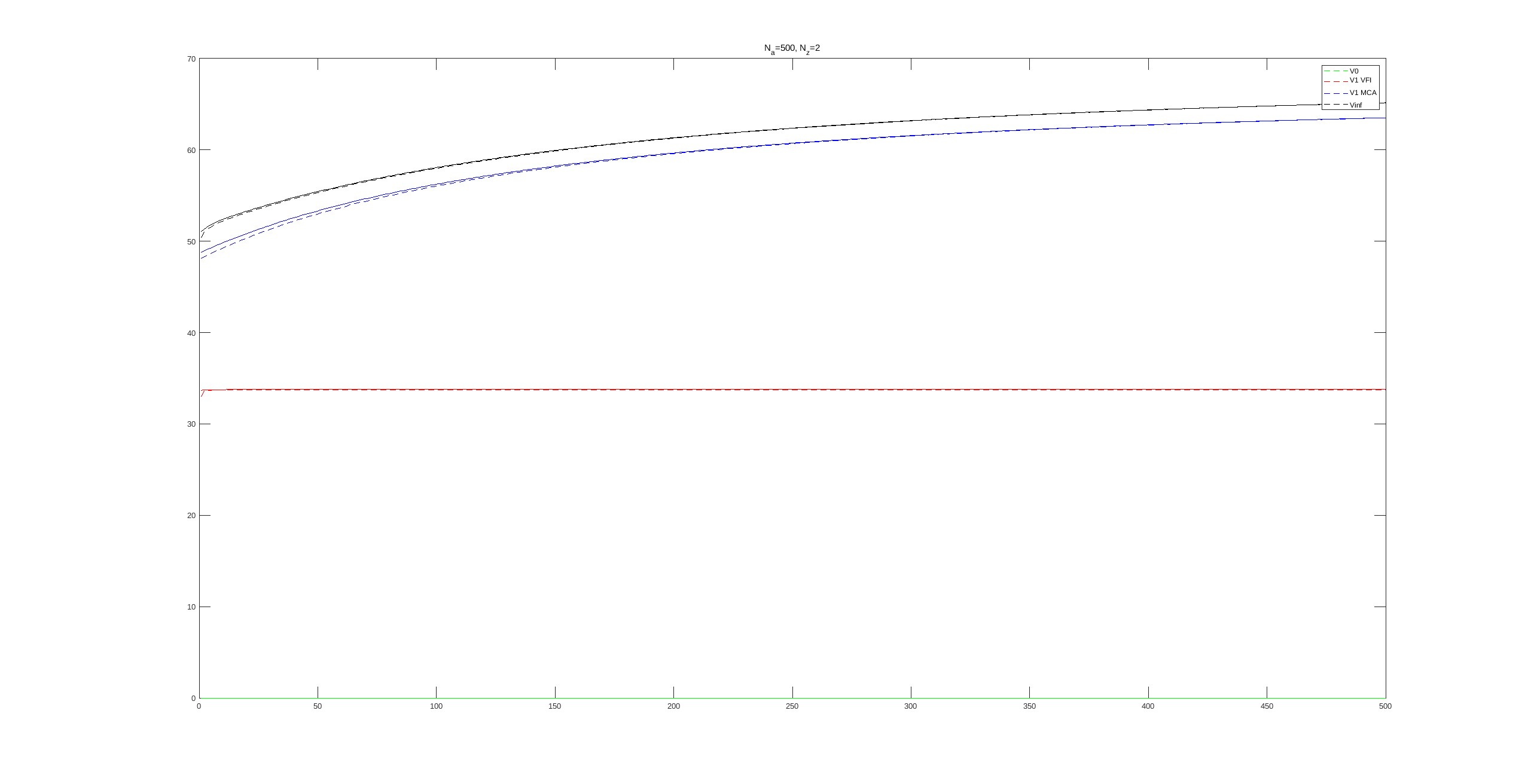
We can also relate all of this to ‘Markov Chain Approximation methods’. Phelan & Eslami (2022) (with corregendium) argue that Markov Chain Approximation methods are a good way to solve continuous time problems, and that implicit finite differences is just one specific example of a Markov Choice approximation method. They also highlight how ‘Markov Chain approximations’ are similar to —but not the same as, see next paragraph— what is here called ‘discretized VFI’ (ignoring that they first have the additional step of getting from the continuous time problem to a discrete time one). For our purposes their point can best be understood as saying that if you solve a discretized VFI there are two main choices (i) you need to choose an interpolation method (they follow the ‘derivatives’ approach like Rendahl; they call this a ‘choice of chain’, their paper is all based on fixed grid spacing but in general this grid is also part of the choice of chain) and (ii) you need to choose whether to use Howards greedy or Howards iteration (they call them PFI and modified-PFI). They illustrate runtimes showing that implicit finite differences (which is Howard greedy, and linear interpolation by derivatives) is faster for small problems, but that switching to Howards iteration is faster for even just a one endogenous state with two exogenous shocks model.
Bakota & Kredler (2022WP) show how to adapt Markov Chain Approximation methods to discrete-time and helps highlight the differences from discretized VFI. Specifically, in discretized VFI we (a) set grid on endogenous state a\_{}grid, (b) set grid and transition matrix for exogenous shocks, z\_{}grid and pi\_{}z, (c) take expectations and interpolate value functions (for aprime values), (d) solve for optimal policy (by a max operation), (e) update the value function. By contrast, for Markov Chain Approximation methods, (c) is done by defining a probability distribution over all points [Note that in discretized VFI if we use linear interpolation we are assigning weights/probabilities to the a\_{}grid and for the expectations we are assigning weights/probabilities to the z\_{}grid; so any difference is just in how the probabilities are assigned, both methods are effectively assigning probabilities to all grid points.] MCA then takes a further step and does a linear moment approximation, taking a first-order approximation of the distribution vector over grid points in the 1st and 2nd moments of the stochastic process. [MCA can if needed take a further approximation of the law-of-motion/return-function.] So we can understand MCA (and the adaptation to discrete time by Bakota & Kredler) as follows: discretized VFI with linear interpolation implemented by the derivatives (the second linear interpolation method described above), with one further ‘linear moment assumption’ (and of course you want to use Howards iteration or Howards greedy).
To understand this linear moment assumption, first consider pure discretized VFI (so next period endogenous state is chosen on the grid). If we model ‘years of education’ as an endogenous state, it is an ‘incremental endogenous state’ as next period/years value is either todays value or todays value plus one (so it can only move by an ‘increment’ of one). Compared to a standard endogenous state where we have n\_{}a values today, and then consider all n\_{}a value tomorrow, an incremental endogenous state is much faster to compute as while we still have n\_{}a values today, we have just 2 values tomorrow; to say the same thing with different words, the state-space is unchanged, but the choice-space is much smaller. The ‘linear moment approximation’ of MCA can here be understood as that the endogenous state is approximated as a bi-incremental endogenous state, so next period value is either the same, or goes up or down one grid point. Now we add the linear interpolation step back in, and we get that the ‘linear moment approximation’ of MCA is to assume that instead of linearly interpolating for all possible next period values, we impose that you can at most go up or down own grid point, so we just have to interpolate for ‘this period grid point and one grid point increase’ and for ‘this period grid point and one grid point increase’. Again, this gives a speed increase (and memory decrease) for the same reason, we keep the same state-space, but massively reduce the next-period choice-space. [Their ‘second’ approximation can be roughly understood as saying if you have two choices, then don’t consider the interaction/cross-term; which is what continuous-time does, always ignoring interactions.] Viewed in this way, the key assumption of the MCA method is that you impose only moving up or down at most one grid point; which cuts runtimes and memory uses, but obviously will be inaccurate if not correct. Note that this (deliberately) looks a lot like the continuous-time assumption, which is that you can only move up or down an epsilon-amount.
More approximation comes with the usual pros and cons, namely faster but less accurate. The main limitation of their linear moment approximation is clearly the requirement that the continuous state does not move up or down more than one grid point in expectation. With one continuous state variable, if the assumption does hold MCA will give the same solution as discretized VFI with linear interpolation (which we know converges to the true solution under standard assumptions). With multiple continuous endogenous states, even when the assumption does hold, the MCA solution will differ subtly from discretized VFI with linear interpolation. There are two tricks that can get the assumption to be more likely to hold (or at least close to holding, so the approximation errors are small). One is to use a coarse grid on the endogenous state —which comes with obvious limits to the accuracy of the algorithm— and the other is to make the model time period very small —which means the discount factor will be larger, which increase the runtimes for infinite horizon VFI problems.
In principle, the ‘bi-incremental endogenous state’ assumption (which they call the ‘linear moment assumption’) is a separate decision to how we do the interpolation, and to the choice of Howards iteration or greedy. So you could do any combination of these. This ‘bi-incremental endogenous state’ is also another way to see what the assumption of continuous-time is implicitly imposing.
A few final details on implementing codes. When doing Howards improvement iteration, the return fn evaluated as the current policy F(a*_m',a_i,z_j) is the same for all iterations h=1,\dots,H, so should be precomputed (it is just a matrix on (a,z)). When doing greedy-Howards improvement T_E is very very sparse, so make sure you set it up as a sparse matrix (T in agent distribution is also very very sparse, but there you want to use the Tan improvement so you won’t create T).
Using Howards iteration (but not greedy) leads to minor differences in the solution to the value function problem, roughly of the same order of magnitude as our solution tolerance (you can see that it leads to different steps in the iteration, so makes sense it might change the solution slighty). This is irrelevant if you just want to solve stationary general equilibrium, but if you want to solve transition paths it can matter, because you will solve the transition path without Howards (Howards doesn’t exist in a finite horizon problem, which is what a transition path is in practice). So if you use the Howards solution, and try to solve a transition path where ‘nothing happens’, those tiny differences in the solution can cumulate over the transition path and result is a tiny non-zero change in policies. As soon as you have any change in policy, the ‘nothing happens’ transition path will blow up. For this reason VFI Toolkit turns off Howards iteration once you get within an order of magnitude of the solution tolerance, so that the final solution is from VFI and not influenced by Howards; increases runtimes very slightly, but becomes more reliable for transition paths. This is implemented in VFI Toolkit code as only doing Howards if ‘currdist/Tolderance>10’.
Using Howards can also be problematic in the first few iterations of VFI. Specfically, if the value of V can contain -\infty then in the first few iterations of VFI these -\infty get spread out around the relevant parts of V. Using Howards, iteration or greedy, while the -\infty are being spread can cause them to be spread to all sorts of places contaminating your value fn with -\infty and breaking everything. For this reason you need to avoid Howards in the first few iterations of VFI if/when the -\infty are being moved around. VFI Toolkit does this by checking that ||V_m(a,z)-V_{m-1}(a,z)|| is finite (so no new -\infty) and only if this is true is Howards used (this is done each m iteration of the VFI). This is implemented in VFI Toolkit code as only doing Howards if ‘isfinite(currdist)’.
One important limitation of Howards greedy is that it will not work for models where the solution V contains some (negative) infinite values. Only for models where V is finite at all points in the state-space. Note that it is okay for the return function to take negative-infinite values, as long as a policy which avoids these can be chosen, and so V remains finite.