De-Gaussing Experiments with ExpAsset

It’s cool that ExpAsset has a kind of built-in graph interpolation, but I didn’t really understand its strengths and weaknesses until I started doing some experiments with it.

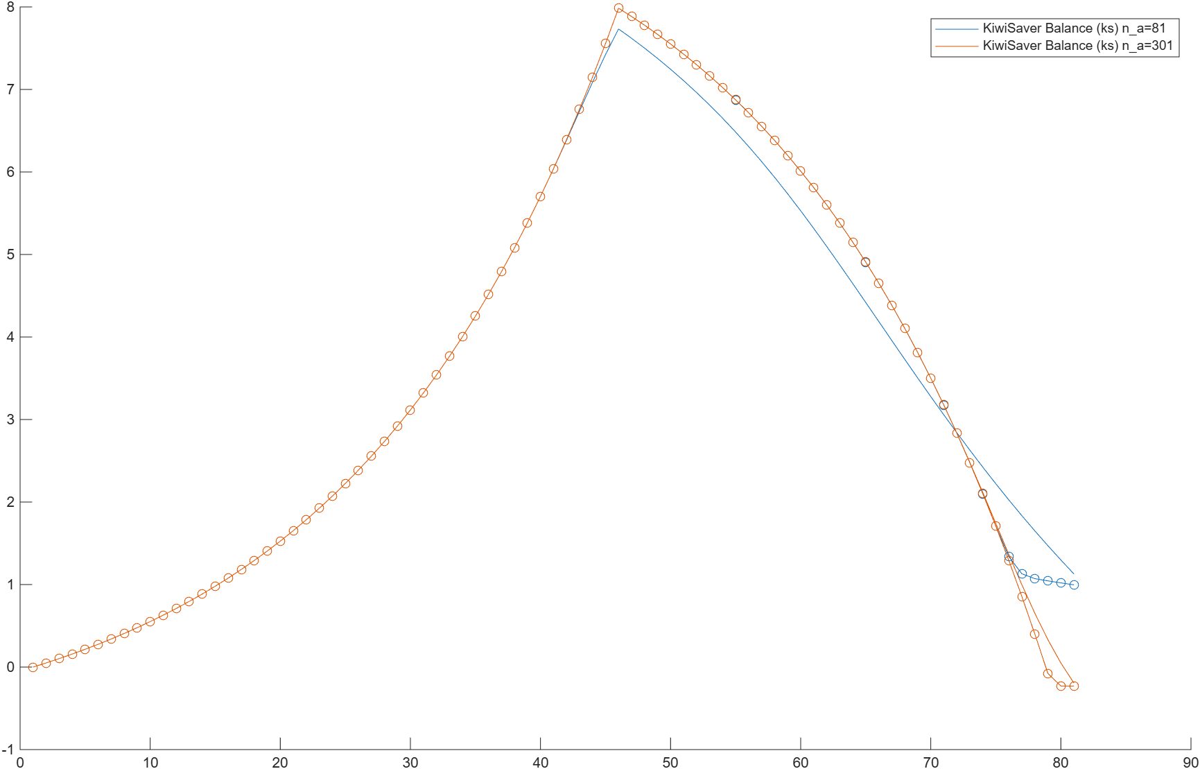
In this experiment, my ExpAsset accumulates contributions of income as well as earning interest, until agej==Jr, at which point the agent withdraws a constant value as a pension while still earning interest on the remaining asset value. I tuned it so that the corpus runs out around model age 79 (modeled age 98).

In this case, 81 grid points (solid blue line) is not enough to accurately trace the evolution of the value of the ExpAsset. But 301 is enough (solid red line, and also red circle line). Is it too much?

The solid blue line is just a graph of the Mean value of the Stationary Distribution (SD) when calculated with 81 grid points (linearly interpolated between -1 and 9 for this model). The blue circle line reads that stationary distribution, cherry-picking those mean values to construct a new a_grid. The idea is that rather than letting the SD do all the work interpolating between our naively chose values, we will carefully curate those values so that the SD probabilities are bang-on 100/0 instead of occasionally 50/50.

The result of this is that we can approximate (up though about age 75) the accuracy of a 301-point grid using only 81 points.

But more than that, consider the problem of computing meaningful Maximum and Minimum values. When the value function returns a value that splits a grid point 50/50, the subsequent period now has two grid points with equal probability. Those grid points might further diffuse the results. Gaussian statistics give us meaningful means, but the Minimum and Maximum values trace the outer edges of this diffusion process. In my experiments, it is typical for the Minimum value to drag down to the bottom of the graph after 8-12 periods (far fewer than by 81 period experiments). Similarly, the Maximum heads off to the top of the graph. Raising the ceiling is not very productive, as the diffusion process grows. Creating a large enough value to capture this supposed (and extremely unlikely) maximum means there’s no precision left over to see what’s happening closer to the mean.

However, when I apply this method of grid interpolation, the Maximum and Minimum values remain well-behaved until very much later. I have not yet done experiments with z and e shocks, which I expect will add some interesting wrinkles. True splitting of probabilities is a different behavior than the Gaussian diffusion I’m solving for. But it may help tame some statistics without resorting to very large grids.
1 Like

I follow what you are saying. The one catch of overruling the default “interpolation onto the two nearest grid points with linear weights” with a “interpolate all weight onto the nearest grid point” is that it leaves a numerical discrepancy between the value fn and the agent distribution.

Whether a numerical discrepency between value fn and agent distribution is better/worse than an outward spread of the agent distribtuion is not an easy question to answer.

Of course all of this goes away if we just put more points on the experience asset grid. But that is not always computationally feasible.

1 Like

I’ve spent some more time observing this diffusion process, and I think this is a fair characterization. Corrections and comments welcomed!

The process of calculating the value function on a finite grid using probabilities to distribute values between two grid points when the value cannot be represented perfectly by one creates a diffusion process that can expand the calculated value by one grid point per generation: one grid point can become two, and the two grid points become three, with the upper and lower grid points creating, respectively, newly expanded upper and lower grid points, while their respective lower and upper grid points sum to a new middle point that is between the new upper and new lower points.

When these excursions ascend or descend beyond the limits of the grid, the values that can no longer be represented evaporate, which becomes an error term.

When the grid is linear, the error term grows by the linear increment value. But how quickly the diffusion reaches the edge is a function of the sum of linear increment values to that edge. Increasing the maximum size of the grid against a linear grid has little reward, as the increase in the cumulative error scales with the maximum value of the grid. Thus the behavior is an imperfect calculation whose cumulative error once reaching the maximum grows as a small fraction of the maximum value of the grid.

When the grid is exponential, the error term grows by the sum of the exponential increment values to the edge, which for the most part means it grows very slowly, leading to a later intercept time. But once the limit is reached, the error term is now the last exponential increment, which is often a substantial fraction of the maximum. This has two implications: (1) if the grid cannot fit the maximum, then the cumulative error after reaching the maximum accumulates more quickly, and (2) by setting a large maximum, the exponential shape can postpone reaching the maximum, perhaps long enough that the larger exponential error term never applies.

For experience assets, we can get accurate calculations by using a reasonably small grid that is scaled to a sufficiently large number that all the probability values fit within the grid and none evaporate. For example, a hypothetical retirement account that grows based on employer and employee contributions at a fixed interest rate can be well-modeled with 17 grid points using a maximum grid value of 36,000 (!). The model calculates a final value of around 19.6 with no shocks and 21.2 with shocks–very small compared to 36,000. But if we use a maximum value of just 56, then almost 15% of the retirement value “evaporates” due to diffusion losses.

With 197 grid points, we only need a maximum grid value of 27 to calculate an accurate retirement value. The lower maximum value is due to the reduced diffusion that 197 affords. But 197 grid points is almost 12x slower and requires 12x more memory (unless one iterates over the experience asset). Thus, a small exponential grid that does not allow escape is a winner.

Adding a reference to a related pull request: Degauss nprobs by MichaelTiemann · Pull Request #114 · vfitoolkit/VFIToolkit-matlab · GitHub

Can you please describe what the pull request aims to implement? Because your above posts just say “I realised that the problem was an artifact of having the grids too widely spaced, and when I cleverly spaced a few grid points the problem went away”, but clearly that is not what the pull request is doing.

EDITED…with progress.

To answer your question: yes, my first attempt at solving the problem was to obviate the need for upper vs. lower by being clever about setting up the grid. When all values land on the grid, there’s no probability leakage to worry about. And yes, I see the limitations of that approach (though it does make one think about more general adaptive grids).

The approach of the pull request is to notice when the Stationary Distribution is getting full of low-probability values and to pull them back into the mainstream. The motivation is that if there’s a very small probability of something happening early on, better to nip it in the bud (which introduces only a small error) than to allow it to create myriad additional low-probability entries that are never remotely possible to reach with the value function. Especially if one has an exponential grid, because the additional gridpoint values grow faster than the assumption of linear interpolation, and things blow up. But this is a bit like chasing horses once they’ve bolted from the stable.

I’m preparing a new pull request based on renormalizing calculations of StationaryDist_jj in the Iteration_nProbs code. Here’s the magic, IF WE HAVE A LINEAR GRID:

Suppose we have StationaryDistribution probabilities evolving like this (which happens if we have an experience asset that’s increasing by 20% on a unit-spaced grid):

11×1 sparse double column vector (2 nonzeros)

   (2,1)       1.0000    % 1.0 is starting value, which happens to be on-grid

11×1 sparse double column vector (2 nonzeros)

   (2,1)       0.8000    % 0.8*1.0
   (3,1)       0.2000    % plus 0.2*2 => Value of 1.2

  11×1 sparse double column vector (3 nonzeros)

   (2,1)       0.6400    % 0.64*1.0
   (3,1)       0.3200    % plus 0.32*2.0
   (4,1)       0.0400    % plus 0.04*3 => Value of 1.4

The first thing we notice is that regardless of the grid magnitude (M) or scale (S), when we look at adjacent points, the value contributed by each point is M+S*(row(n)-row(1)+1). In matlab:

% values are the coefficients of the non-zero StationaryDist_jj terms
multipliers=(0:row_idx(end)-row_idx(1))'+1;
ea_value=sum(values.*multipliers)

In the default implementation, we compute a Gammatranspose that accumulates values at repeated indexes, but for this case I keep the lower grid and upper grids separate across the Gammatranspose:

II1=(1:1:N_a)';
for jj=1:(N_j-1)
    % ignoring regular Gammatranspose and StationaryDist_jj for clarity
    Gammatranspose_lower=sparse(Policy_aprime(:,1,jj),II1,PolicyProbs(:,1,jj),N_a,N_a);
    Gammatranspose_upper=sparse(Policy_aprime(:,2,jj),II1,PolicyProbs(:,2,jj),N_a,N_a);
    StationaryDist_lower_jj=Gammatranspose_lower*StationaryDist_jj;
    StationaryDist_upper_jj=Gammatranspose_upper*StationaryDist_jj;

    [row_lower_idx, ~,lower_values]=find(StationaryDist_lower_jj);
    multipliers_lower=(0:row_lower_idx(end)-row_lower_idx(1))'+1;
    if nnz(StationaryDist_upper_jj)
        % Attempt to consolidate upper into lower
        [row_upper_idx,~,upper_values]=find(StationaryDist_upper_jj);
        multipliers_upper=(row_upper_idx(1)-row_lower_idx(1):(row_upper_idx(end)-row_lower_idx(1)))'+1;
        sum_upper=sum(upper_values.*multipliers_upper);
        if sum_upper/multipliers_lower(end)+lower_values(end)<=1
            % We can fit all the upper values into slots allocated to lower...
            lower_values(end)=lower_values(end)+sum_upper/multipliers_lower(end);
            % But in so doing, we may have probabilities that sum>1, so fix
            lower_values=linsolve([multipliers_lower';ones(1,length(lower_values))],[sum(lower_values.*multipliers_lower); 1]);
            % Clean up linsolve rounding errors at zero and 1
            lower_values=round(lower_values(lower_values<=1e-6 | lower_values>=1-1e-6));
            StationaryDist_jj=sparse(row_lower_idx,1,lower_values,N_a,1);
   end
   % StationaryDist(:,jj+1)=gather(full(StationaryDist_jj));
end

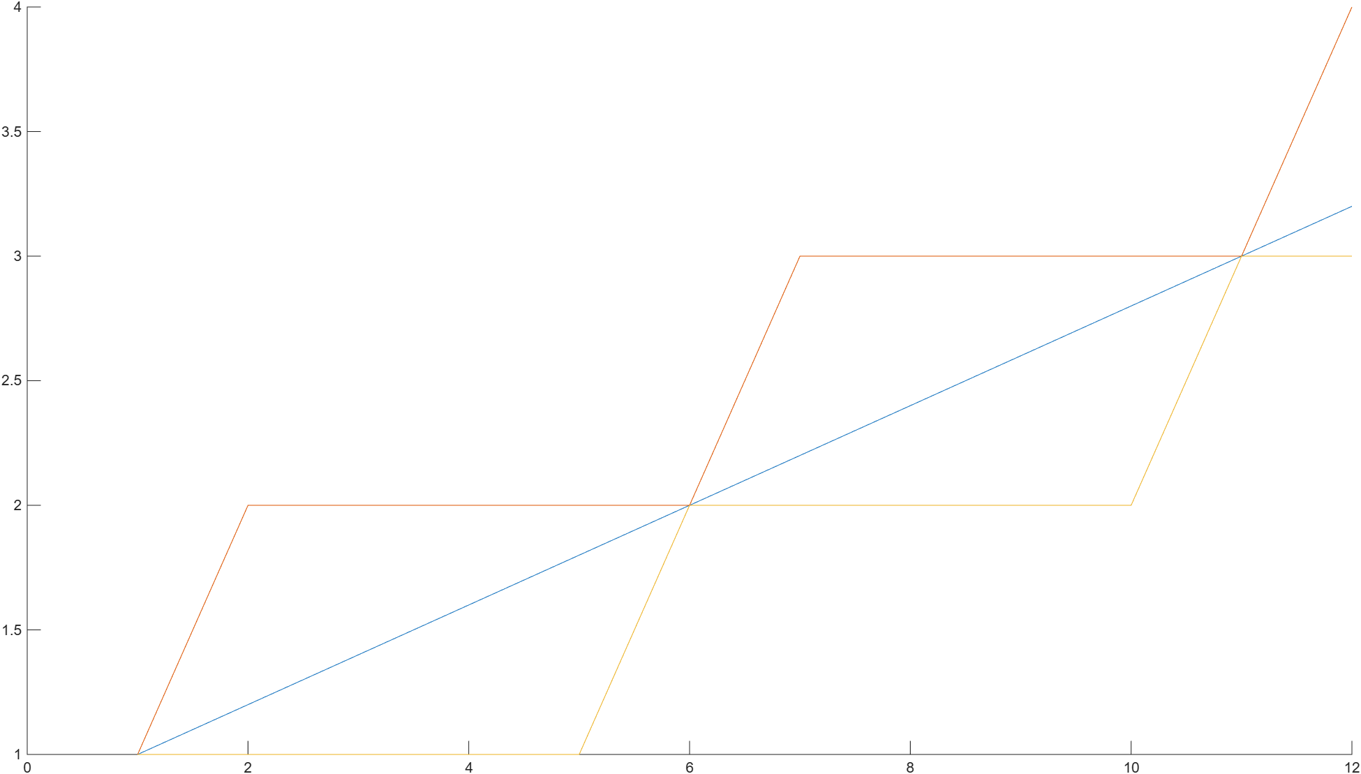
Let’s compare the result in pictures:

Original behavior, showing evolution of experience asset (in blue) with maximum (red) and minimum (yellow). Note that the maximum value increases one grid value at each step.

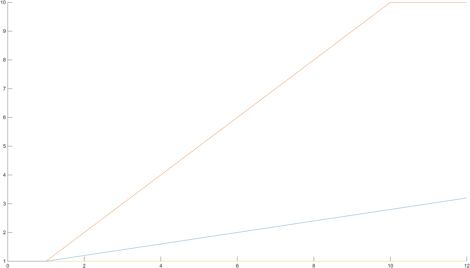
Now, using the linear equations solver:

Notice that the maximum and minimum follow the maximum and minimum involved gridpoints.

This was my goal.

I think I see what you are saying. There could be a simoptions setting a threshold when doing linear interpolation back onto the grid while simulating agent distribution.

Threshold would work as follows: We linearly interpolate a choice a^* onto the points a_i and a_{i+1}. This involves putting p on a_i and 1-p on a_{i+1}. If p is less than the threshold, then overwrite with putting 0 on a_i and 1 on a_{i+1} (and analogously if 1-p is less than the threshold).

This would be an option, but is not something that would be the default. It does a behaviour a user might plausibly want, but very much a second-best behaviour relative to just adding more grid points.

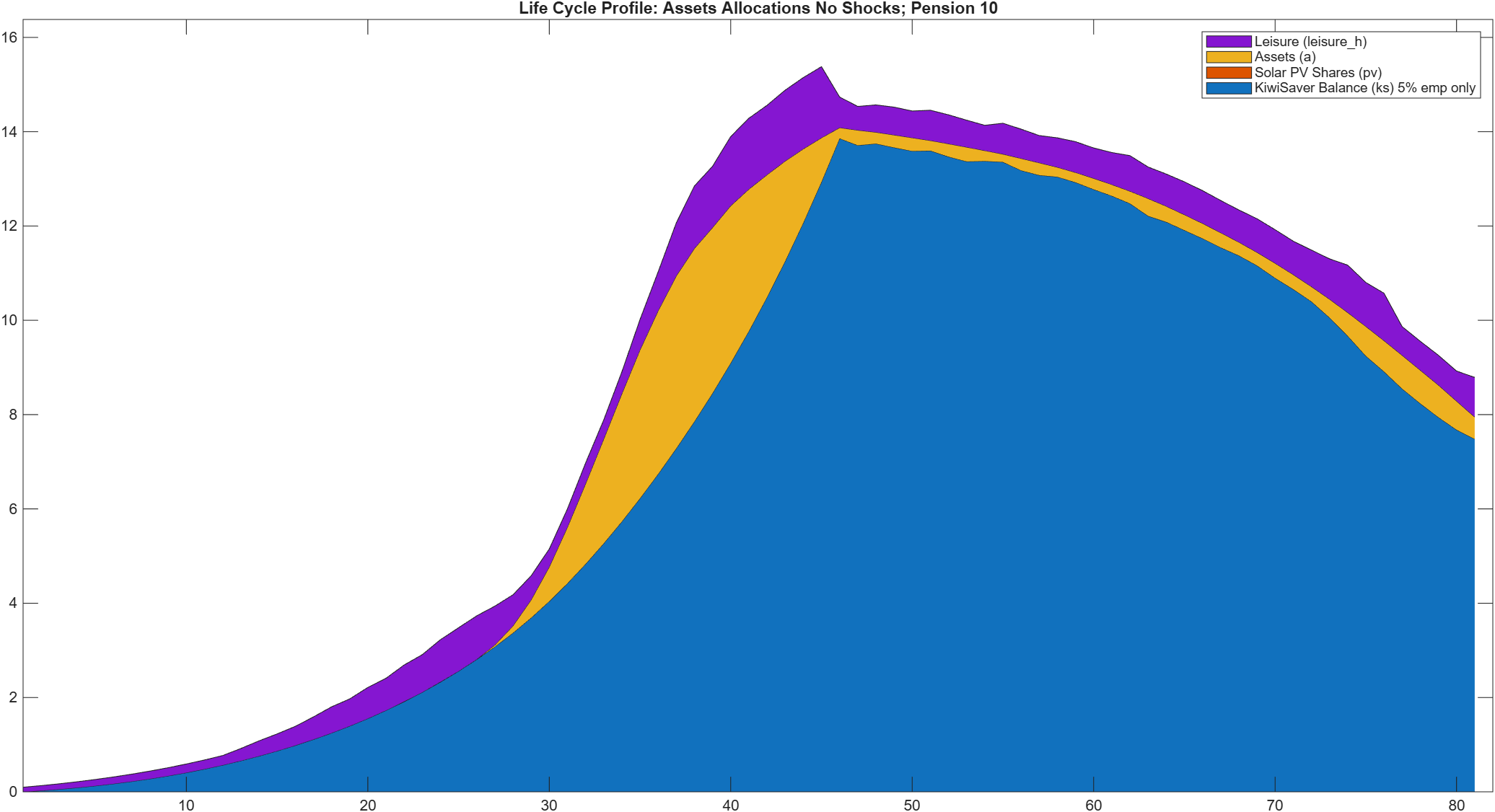
I think the change is rocket :rocket: fuel for experience assets. I think it will be possible to get accurate results with very few gridpoints, reducing the curse of dimensionality. We’ll see…
It is doing to add distortion to the mean, but reduce distortion of higher order moments.

I’ll add right now that the grids of my simple test (noa1, noz) are appropriate for demonstrating the example. But when we have additional assets, not to mention possible z and e terms, the calculations to pick multipliers out of StationaryDist_jj row numbers requires some work. I will investigate that before proposing a new pull request.

I have it half-working (deposits to retirement account look rational). The half that’s not working is when agent make withdrawals. But lots of interesting edge cases.

For example, zero-valued coefficients may appear, and we want to let them bubble out. Fortunately, the linear solver can make quick work of that: if we have X11+02+X33 we don’t know that we can fit X33 into the X22 slot (we might run out of probability space if X1+X2 is greater than the total probability allocated to the slice). But we do know we can fit X11 into the X2 slot, because X2 has a multiplier of 2, and an X1 that works with a multiplier of 1 can fit when we cut its probability value in half. The linear solver can then redistribute the values between X2 and X3 so that the sum of the probabilities of X2 and X3 total to whatever the slice requires. And then we get the correct value when we multiply the gridvals by the respective probabilities.

On to fix withdrawals!

Can you say more about adding distortion to the mean? The mean graphs I posted show the mean tracking as expected. Since those posts, I’ve uncovered some other logical errors in the simple that I’ve fixed, and now I have good results whether the grid has 10 points for every incremental value or one point for every 10 values. (Previously changing grid densities pointed out where edge cases were not being correctly handled.)

But I am tracking down some anomalies in more complicated examples, and if I can better understand what you mean, I can either sharpen my focus while fixing them, or relax my expectations. Thanks!

Repeat: Threshold would work as follows: We linearly interpolate a choice a* onto the points a_i and a_{i+1}. This involves putting p on a_i and 1-p on a_{i+1}. If p is less than the threshold, then overwrite with putting 0 on a_i and 1 on a_{i+1} (and analogously if 1-p is less than the threshold).

New: Say a*=5.9, a_3=5 and a_4=6.

If we do the standard linear interpolation we get p=0.1 at a_3 and 1-p=0.9 at a_4. So for the mean we have p*a_3+(1-p)*a_4=0.1*5+0.9*6=5.9 so the mean is exact. While for the variance we will get >0 while the exact is 0; note that we can get this error in the variance to go to zero by moving the two grid points closer together.

Now do linear interpolation with ‘threshold’ of 0.2 (bigger than we would likely ever set, but just pretend). Now p=0.1 is below threshold, so overwrite with 0, and thus we get mass of 0 at a_3 and mass of 1 at a_4. So now the mean is 6, which is worse (exact would be 5.9) but the variance is zero (which in this heavily cooked example is exact). So using the threshold made the mean worse, but improved the higher order moments.

[One way to think about this is that standard linear interpolation is build around focusing on getting the mean correct.]

Thanks for that explanation. I wasn’t thinking about the consequences of the threshold implementation. I was only looking at using linear solutions to reformulate the means with fewer variables as the experience asset evolves.

The implementation I’m striving for preserves both the mean value exactly and the probabilities within the slices of the stationary distribution (both as to ze variables and as to all the non-experience asset states). It’s true that the variance of the experience assets may change, as I can keep the values as close to the mean as the grid permits (rather than growing with every generation).

I’ll keep working to show I have it right for both the simple case (nod, noa1, noz) and a more complicated one (with d, multiple a, and z).

Success is getting closer! I just needed to learn how to spell:

StationaryDist_jj(sub2ind([N_a1,N_a2,z_c],col,row_lowerz_idx(1):row_upperz_idx(end),z_c))=StationaryDist_lowerz_jj(row_lowerz_idx(1):row_upperz_idx(end),col);

Here’s a progress graph…finally smooth on the way up and the way down.

However, we are still not shrink-wrapping the maxima as we do in the toy example. And when the size of the graph spacing is 3x larger, things go haywire. So I probably still have a few index/logic errors to find and fix. But it feels very doable now.

I’ve been watching my Stationary Distribution evolve over 5 steps. In the first four steps the reshaped elements encode the mean with an error around 1e-6 compared with the return function. On the 5the step, the error jumps to 0.0025. I suspect the reason is because the Tan improvement depends upon an implicit structural link between the (backwards) Policy_aprimez/PolicyProbs construction and the (forwards) StationaryDist_jj construction.

Here are the relevant PolicyProbs for jj=5:

K>> yy=reshape(PolicyProbs,[197,37,2,2,81]);
K>> yy(66,1:5,1,:,5)

  1×5×1×2 single array

ans(:,:,1,1) =

    0.9158    0.8458    0.7758    0.7058    0.6358


ans(:,:,1,2) =

    0.0842    0.1542    0.2242    0.2942    0.3642

gg=reshape(full(Gammatranspose),[N_a1,N_a2,N_z,N_a1,N_a2,N_z]);
gg1=squeeze(gg(:,:,1,:,:,1));
gg1(66,1:5,66,1:5)

They sum to 1 vertically, and the piece of the Gamma Transpose that applies for the lower grid ans(:,:,1,1) is a diagonal matrix that begins [0.9158 0.8458 0.7758 0.7058 0.6358] down the “eye”, while the piece that applies to the upper grid is a diagonal just below that containing [0.0842 0.1542 0.2242 0.2942 0.3642].

Coming into the Tan improvement StationaryDist_jj actually holds data from jj=4

zz=StationaryDist(:,jj);
zz=reshape(zz,[N_a1,N_a2,N_z]);
zz=zz(:,:,1)';
zz(1:4,66)

ans =

  4×1 gpuArray single column vector

    0.8144
    0.1612
    0.0227
    0.0017

The shape of the Stationary Distribution grows a row each age step; the Gammatranspose multiplication grows it to 5 elements:

% After multiplying by Gammatranspose
zz(1:5,66)

  5×1 gpuArray single column vector

    0.7507
    0.2010
    0.0416
    0.0062
    0.0005

K>> sum(zz(1:5,66).*ks_grid(1:5))

ans =

  gpuArray single

    0.1267

The 0.1267 number is the target.

I’m trying to make the evolution of the Stationary Distribution more compact. Coming into the Tan improvement my age==4 matrix is:

ans =

  3×1 gpuArray single column vector

    0.6952
    0.3048
         0

Note that the probabilities sum to 1 and the weighted probability sum gives the correct answer for aprime when jj==4. After the Tan improvement the Stationary Distribution becomes

StationaryDist_colz_jj =

  37×197 sparse single matrix (3 nonzeros)

   (1,66)      0.6367
   (2,66)      0.3163
   (3,66)      0.0470

and this is where we overshoot the value of aprime by 0.0025 (giving 0.1706).

I had naively thought that the Gammatranspose matrix provided a set of facts about (a',z) and that would “just work” when used as a multiplier against any properly constructed Stationary Distribution. Am I doomed or is there a correction I can apply?

If you are trying to do the ‘threshold’ approach, you should simply edit PolicyProbs directly.

I’m actually trying to do something different. I’m trying to achieve an exact result by managing the forward evolution of the Stationary Distribution more carefully. I feel like there is a way to do it…I just need to find the right seam in the rocks.

I figured out my instant problem! (I will edit for clarity once I get something working)

I adjust the Stationary Distribution along these lines:

temp=sparse(row_lowerz_idx,col,lowerz_values,N_a2,N_a1); % Note transposed!
temp_rows=row_lowerz_idx(1):row_upperz_idx(end);
StationaryDist_jj(sub2ind([N_a1,N_a2,z_c],col,temp_rows,z_c))=temp(temp_rows,col);

Originally I started by splitting the distribution into lower and upper grids, but I’ve put on my todo list doing everything against a unified grid. In any case, with the split grids…

  • col indexes into where we are in N_a1
  • the rows are experience asset indices

When I notice that I can move all the values from one grid to slots allocated to the other (using linsolve to adjust the probabilities), I put the useful lower or upper grid back into the Stationary Distribution and the Stationary Distribution forgets ever needing the other grid. All the probabilities and all the means are as close floating point arithmetic allows.

The good news is that at this point in the code I have all the handles I need to update Policy_aprimez and PolicyProbs: I know the a1 index (it’s col), the a2 indexes (they are temp_rows), the z index (it’s z_c), and the age (it’s jj). And since I’m working from split grids, I know my lower from my upper. So I should be able to patch up the probabilities and re-run the process with a Gammatransform that gives me the correct lower and upper grids a second time around. That second time around is trivial–we’ve done all the heavy lifting and now we just need to calculate the stationary distribution as per usual.

I’m going to give it a try…

P.S. Maybe the split grid start wasn’t such a bad idea…we’ll see.

Looking good up to here. The REFERENCE shows how the values spread across the stationary distribution with Gaussian diffusion. The NEW shows the tight construction. Row 38 is the weighted sum of the experience asset grid.

Age jj = 17; REFERENCE

ans =

  38×1 sparse single column vector (22 nonzeros)

   (2,1)       0.0772
   (3,1)       0.1442
   (4,1)       0.1794
   (5,1)       0.1847
   (6,1)       0.1692
   (7,1)       0.1428
   (8,1)       0.1130
   (9,1)       0.0843
  (10,1)       0.0596
  (11,1)       0.0398
  (12,1)       0.0250
  (13,1)       0.0147
  (14,1)       0.0081
  (15,1)       0.0037
  (16,1)       0.0015
  (17,1)       0.0005
  (18,1)       0.0002
  (19,1)       0.0000
  (20,1)       0.0000
  (21,1)       0.0000
  (22,1)       0.0000
  (38,1)       1.2478

NEW

ans =

  38×1 sparse single column vector (4 nonzeros)

   (3,1)       0.1962
   (4,1)       0.6577
   (5,1)       0.3937
  (38,1)       1.2476

At Age 20, Policy_aprimez changes:

K>> squeeze(Policy_aprimez(66+197*(0:5),1:2,19))

ans =

          66         263
         263         460
         460         657
         657         854
         854        1051
        1051        1248

K>> squeeze(Policy_aprimez(66+197*(0:5),1:2,20))

ans =

          66         263
         263         460
         461         658    % 658 ~= 657
         657         854
         854        1051
        1051        1248

What does this mean? (Omitting z_c for clarity)

K>> [row,col,z_c]=ind2sub([N_a1,N_a2,N_z],657)

row =

    66

col =

     4

K>> [row,col,z_c]=ind2sub([N_a1,N_a2,N_z],658)

row =

    67

col =

     4

It means my agents have moved the ground under my feet…