Notes on supporting exponential grids for probability re-distribution

[MichaelTiemann]

This is a note to myself about how to support non-linear grids, not only linear grids, when redistributing probabilities. I have found good success wrangling probabilities on linear grids, but some of my problems are better represented by exponential grids. I remembered enough linear algebra to solve the linear grid problem, but got lost trying to solve the exponential grid problem. This is what Gemini told me…

When you transition from isolated expected values to full distributions with distinct, non-overlapping clusters of probability, the most robust approach is to handle the mapping and reduction locally. This ensures you maintain the shape, mass, and expected value of each individual cluster without bleeding probability across the entire grid.

Here is how you can translate these clusters to your exponential grid Y = \exp(0:\ln(N+1))-1, and subsequently reduce them.

1. Translating Clusters to the Exponential Grid

To translate clusters from your linear grid X to the exponential grid Y, you apply the adjacent-point projection method point-by-point rather than globally. This preserves the local expected value of every individual element in your clusters.

For every point x_k in a cluster on grid X that has a probability p_k > 0:

1. Find the two adjacent points y_m and y_{m+1} on the exponential grid such that y_m \le x_k \le y_{m+1}.
2. Split the probability p_k between these two points to preserve x_k’s expected value contribution:

q_{m+1} = p_k \frac{x_k - y_m}{y_{m+1} - y_m}

q_m = p_k - q_{m+1}

3. Sum the overlapping probabilities on the Y grid. If a translated point from one cluster overlaps with another (which is possible depending on the resolution of Y), you simply add the assigned probabilities together at that grid node.

This step guarantees a feasible, non-negative distribution on the exponential grid that perfectly preserves both the total probability (1.0) and the global expected value, while keeping the structural “clusters” intact.

2. The Reduction Step for a Cluster

Once your probabilities are translated to the exponential grid Y, you might find that a cluster spans several consecutive grid nodes (e.g., from index a to index b).

To reduce this cluster to a “minimal basis” representation on the exponential grid, you compress the entire cluster down to its two local endpoints: y_a and y_b.

First, calculate the total mass and the expected value of this specific cluster:

• Cluster Probability (p_c): \sum_{i=a}^{b} q_i
• Cluster Value (V_c): \sum_{i=a}^{b} q_i y_i

Next, set up the linear system for the new reduced probabilities, q_a' and q_b', at the endpoints of the cluster:

\begin{bmatrix} 1 & 1 \\ y_a & y_b \end{bmatrix} \begin{bmatrix} q_a' \\ q_b' \end{bmatrix} = \begin{bmatrix} p_c \\ V_c \end{bmatrix}

Solving this system yields the reduction formulas:

q_b' = \frac{V_c - p_c y_a}{y_b - y_a}

q_a' = p_c - q_b'

Why this is Always Feasible

In your previous global example, feasibility was an issue if the expected value escaped the grid bounds. For local cluster reduction, it is mathematically guaranteed to be feasible (no negative probabilities).

Because V_c is the expected value strictly derived from the points between y_a and y_b, the “center of mass” of the cluster (\frac{V_c}{p_c}) will always fall strictly between y_a and y_b:

y_a \le \frac{V_c}{p_c} \le y_b

If you multiply that inequality by p_c, you get:

p_c y_a \le V_c \le p_c y_b

Because V_c is guaranteed to be greater than or equal to p_c y_a, the numerator in the q_b' equation (V_c - p_c y_a) will always be positive, guaranteeing that both q_a' and q_b' are valid, non-negative probabilities.

You can apply this exact reduction step independently to the run of probabilities at i:i+3 and the run at j:j+4, compressing each into just two non-zero grid points on the exponential grid.

[MichaelTiemann]

Sheesh…I was so close I probably actually tried this very thing, but something else wasn’t working and that was clouding my analysis as to what was or was not working.

The problem, for you Linear Algebra nerds, was that the code I wrote to try to create zeros was flawed. I created a vector, zero_candidates that kept track of the zeros I was trying to create.

The optimization tries to knock down the probability stored at the maximum index by reallocating it amongst lower index levels. When there’s no more to push down from the top, it tries pushing up the minimum to redistribute among the remaining higher index levels. I have posted elsewhere the graphs showing the effectiveness of this “shrink-wrapping”.

But here’s what i got wrong. I wrote

SystemOfEquations=[a2_grid(this_run(nonzeros))';ones(1,nnz(nonzeros));zero_candidates(nonzeros)];
GoalValues=[sum(vals(nonzeros).*a2_grid(this_run(nonzeros))'); run_prob_sum; 0];
new_vals=linsolve(SystemOfEquations,GoalValues);

When zero_candidates is something like [1 0 0 0 1] what I was trying to say is that we are constraining the min and and the max to be zero. But of course what I said was “the probabilities at the min and max indices must sum to zero”, sometimes resulting in a pair of zeros, but often resulting in a pair of numbers that summed to zero. What I should have written was:

ZC=eye(nonzeros,nonzeros).*zero_candidate(nonzeros);
ZC=ZC(any(ZC~=0,2),:);
SystemOfEquations=[a2_grid(this_run(nonzeros))';ones(1,nnz(nonzeros));ZC];
GoalValues=[sum(vals(nonzeros).*a2_grid(this_run(nonzeros))'); run_prob_sum; zeros(size(ZC,1),1)];
new_vals=linsolve(SystemOfEquations,GoalValues);

This creates an equation for each index I’m trying to set to zero, which is what I meant to say

Progress continues…

[MichaelTiemann]

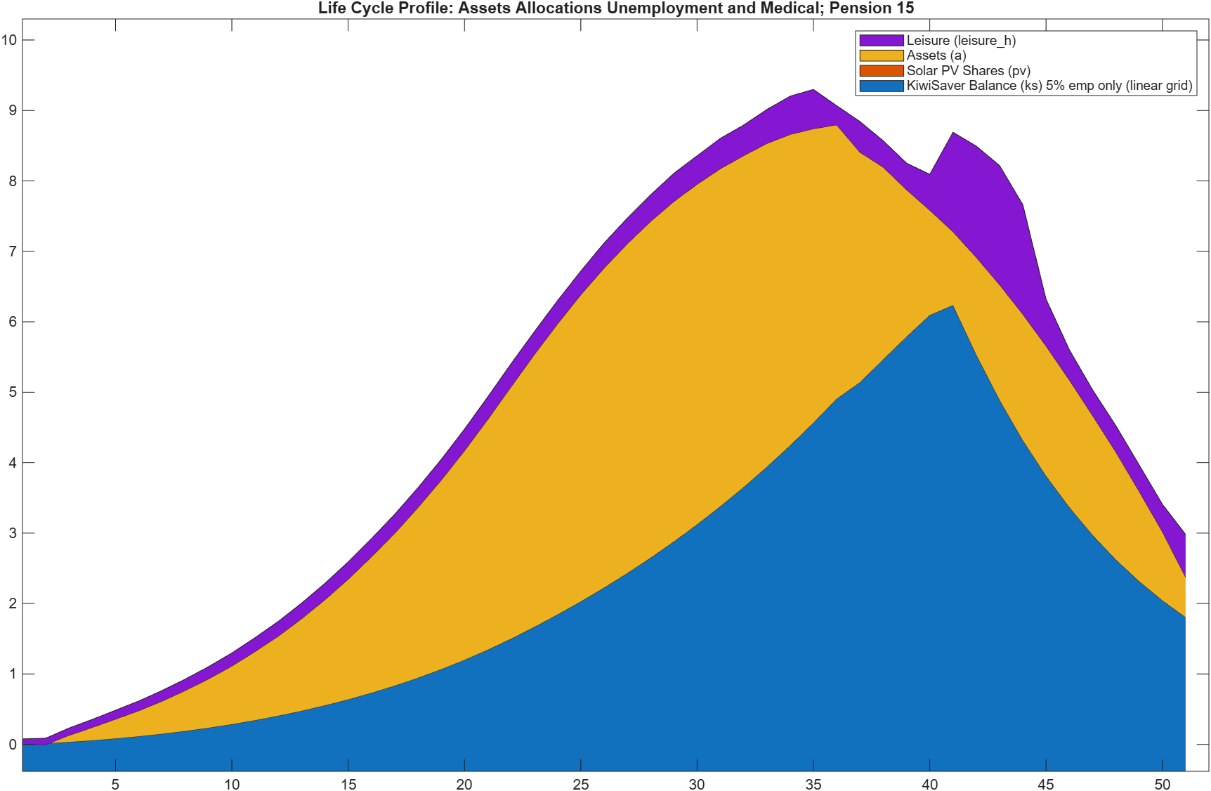
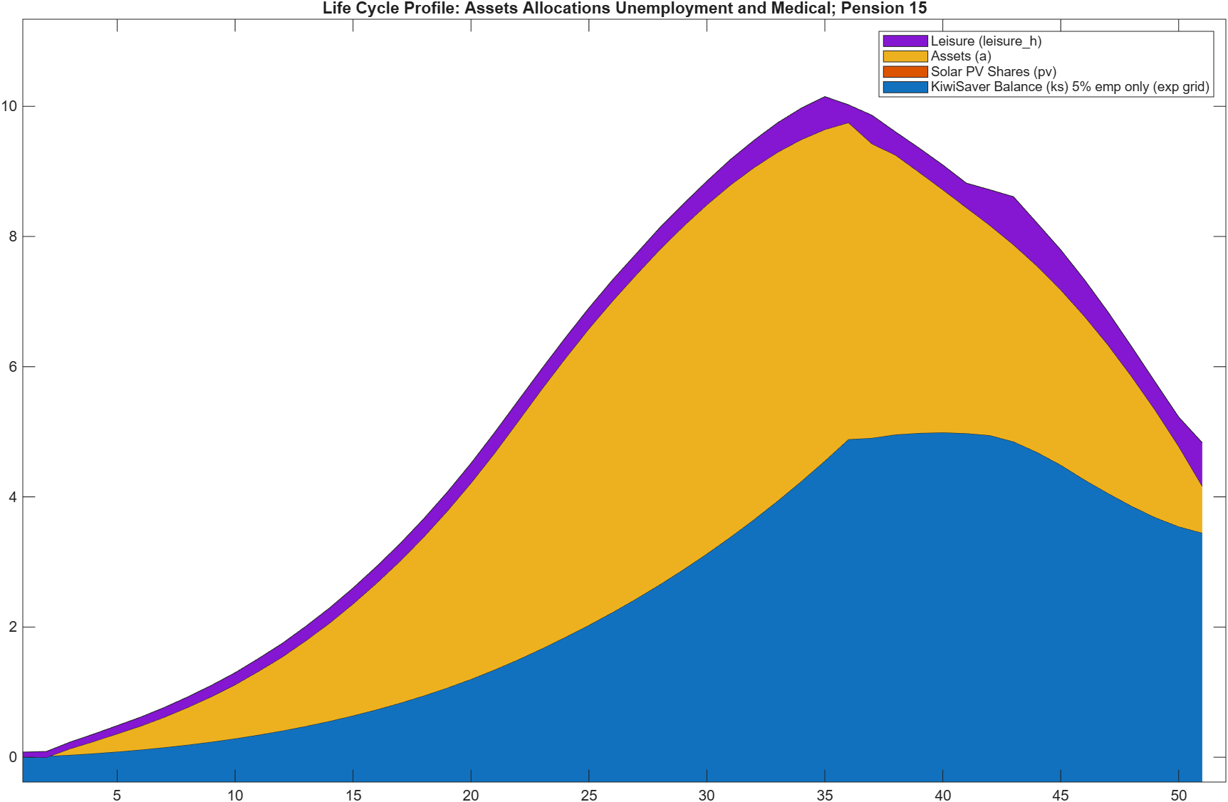
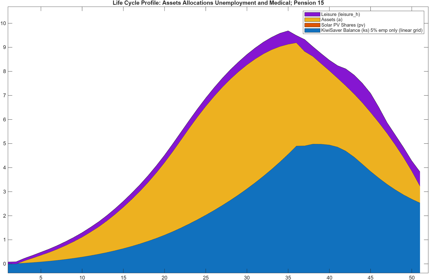
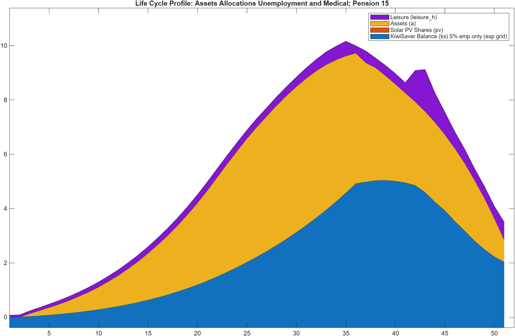
I think I am now supporting both linear and non-linear grids now. Here are some examples (all of which derive from LifeCycleModel21 but enhanced with a savings plan and some other features).

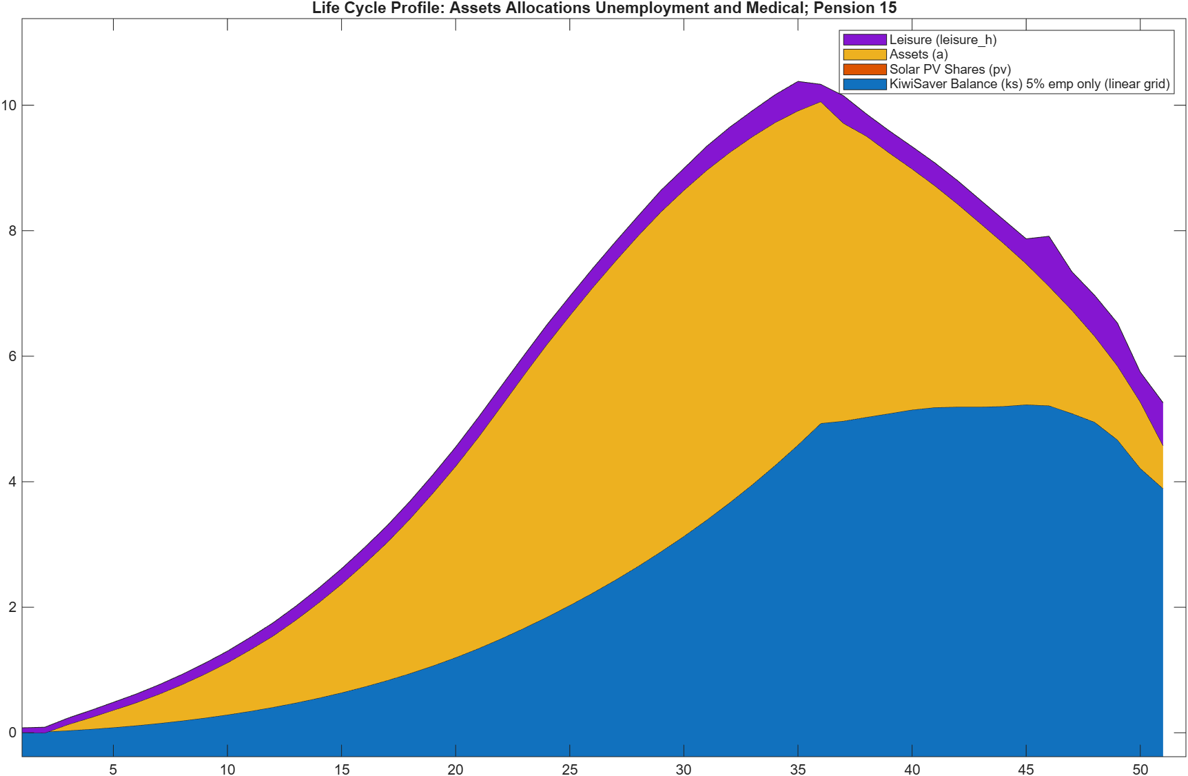
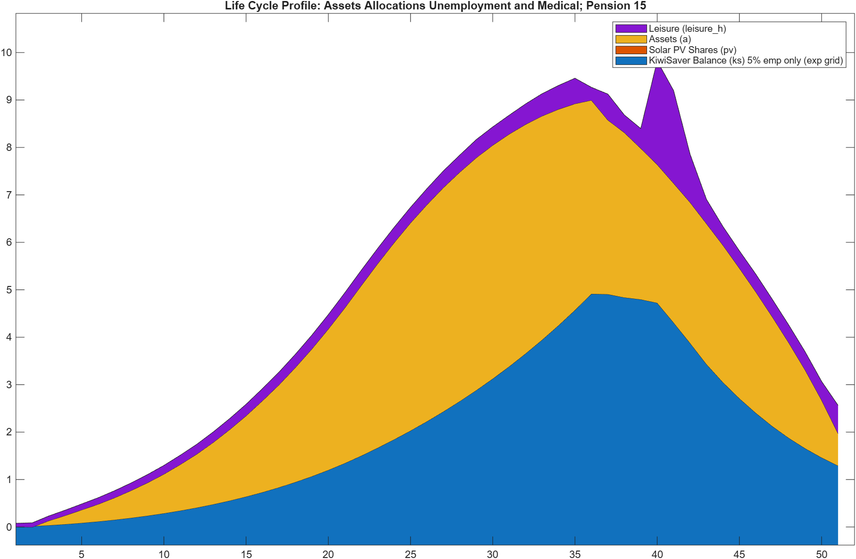
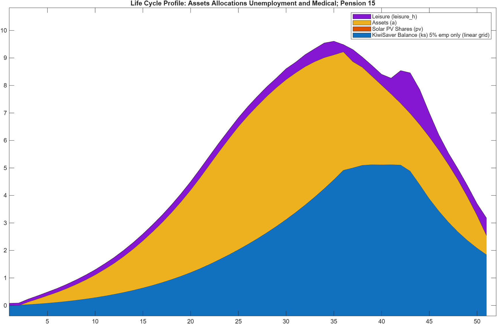
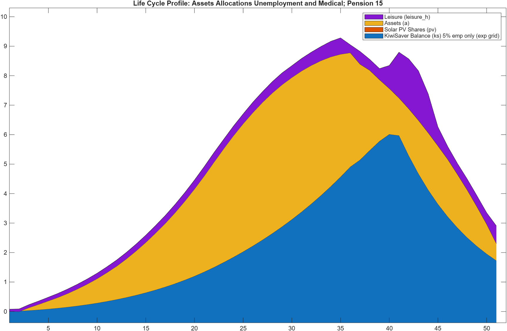
I think this shows that the exponential grid gives a more accurate picture sooner as to the behavior of the experience asset. I chose three grid sizes to compare: 17, 57, and 196. Here they are:

With a grid size of 17, the exp grid (top image) is more hump-shaped.

With a grid size of 57 we see both humps begin to narrow. The linear shape at 57 begins to look like the exp shape at 17.

With 197 grid points the two very much begin to agree.

[MichaelTiemann]

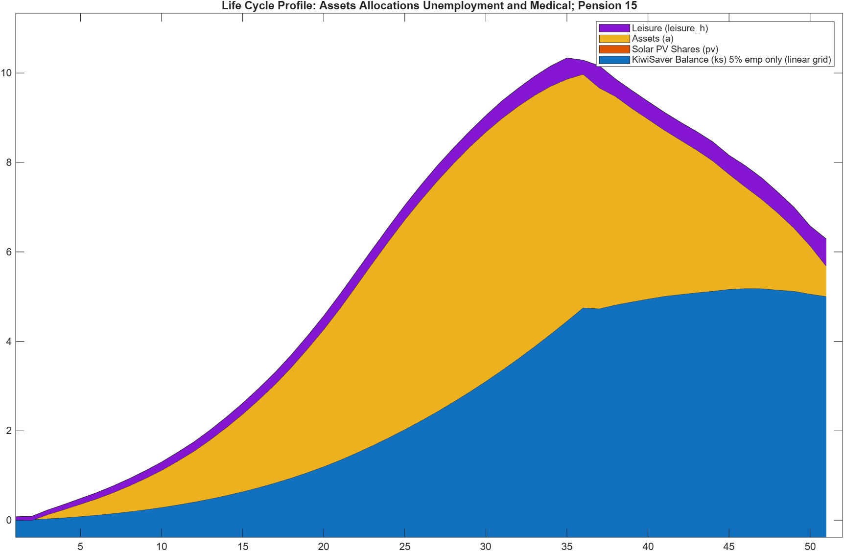
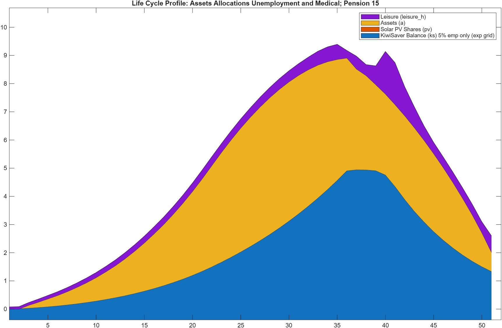
Without the nProbs optimization, 17 grid points is definitely not enough. The exponential grid is a little better than the optimized linear grid, but not by much.

The linear grid mostly loses its hump.

With 57 grid points, the non-optimized exp grid looks very much like the optimized one of the same size.

The linear grid shows a larger difference compared to the 57 grid points optimized.

The intention of the optimization is to make it more practical to use smaller-dimensioned experience assets in modeling. Exponential grids help!

[MichaelTiemann]

Note that the examples above live on a shortened lifecycle horizon. I shifted the age shifter by 10 years, and I shortened the lifespan from 100 years to 80, providing only 50 years of model time. When I returned the model to its full timeline…

At 997 gridpoints for the experience asset, both exponential and linear agree extremely well, once the proper maximum value is set (in this case 20). As the grid maximum grows, the linear grid starts to lose its grip.

20 - “perfect” agreement

50 - excellent agreement

100 - good agreement

200 - 50% excess value at the end

500 - start of exponential runaway (hump shape is a plateau)

1000 - full exponential runaway; the grid doesn’t have enough points to prevent upper gridvals from reaching the top of the grid and creating havoc.

When we drop to 197 gridpoints, we find for these maxvals:

20 - good agreement

50 - more than 100% excess value at end

100 - start of exponential runaway (hump shape is a plateau)

Alas, that’s where we hit our ceiling for the linear grid, because we need about 10 grid points per value to keep from getting caught in the exponential runaway. The exponential grid gives good results down to 97 grid points, then starts getting wobbly, a 2x improvement.

With optimize_nProbs, the linear grid actually shows better with 97 than the exponential. Indeed the linear graph looks good down to 37 gridpoints, and even 29 if we further fine-tune the maxval down to 16.

All this to say: of course it matters the size and shape of one’s grids when it comes to getting accurate results. But sometimes an exponential grid can offer a 2x performance boost and sometimes linear algebra can offer a 7x improvement, give or take.