Good spot. Just updated to fix.
1 Like
I think there is a typo in the assets plots. The policy function a'(a,z) for a given z should be convex in a since the policy for consumption is concave.
Moreover the policy for a’ given z1 should have a flat part for small values of assets, where the borrowing constraint binds.
Spotted: You are not using PolicyVals in the plots
Good spot! I have corrected the above assets plots to use PolicyVals, and corrected the code.
On the convexity, it is there, just hard to see as there is only a small amount of convexity. Here is a graph, same as the above but zoomed in at low assets (and dropping the ‘zsuper’ as it otherwise makes the graph hard to read),
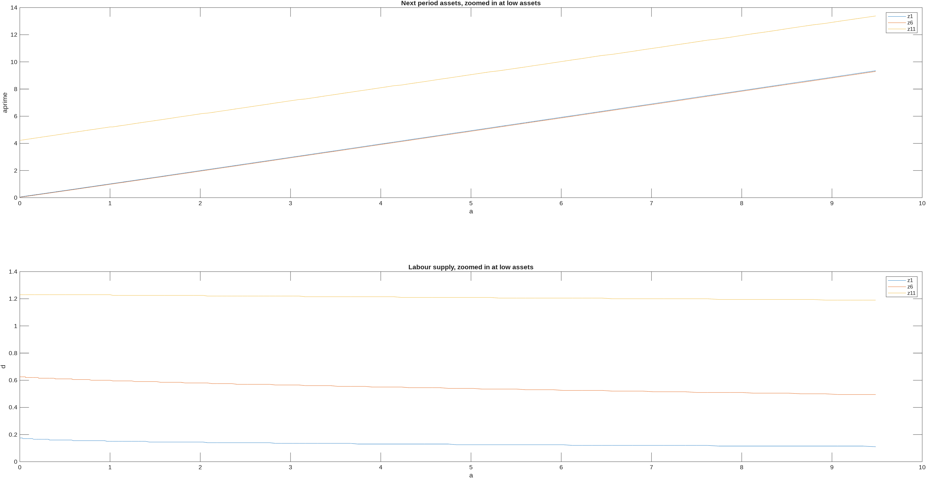
you can see in the top panel that assets is convex (if you look really closely), but it is only a little bit convex and the bottom panel shows why, namely there is a fair bit of ‘precautionary labor supply’ which reduces the need for ‘precautionary savings’ (Pijoan-Mas, 2006).
Here is another graph, this time zooming in even more on low assets and only for the lowest worker productivity z1, which plots both next period assets (optimal policy) and a straight line connecting the two ends of the next period assets,
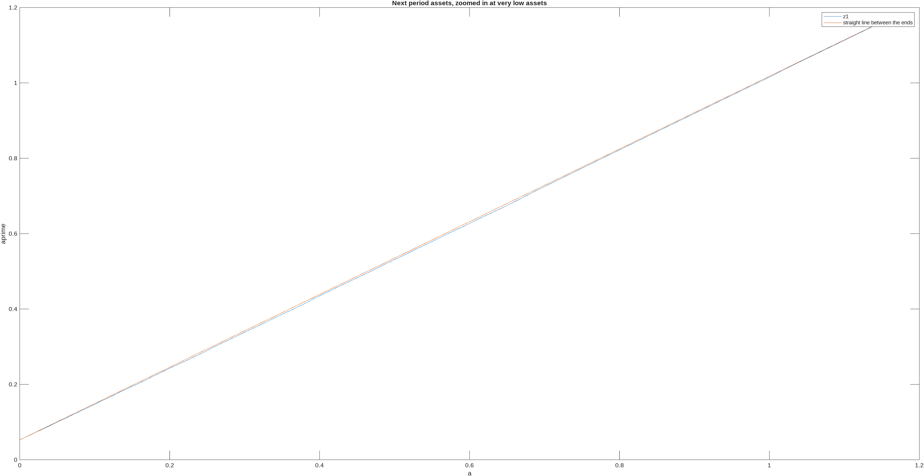
you can see that the straight line is above the next period asset optimal policy, illustrating that it is convex.
Here is code for these two additional graphs (that uses PolicyVals created in code in earlier post)
figure_c=figure_c+1;
figure(figure_c);
subplot(2,1,1); plot(a_grid(1:200),PolicyVals(2,1:200,1),a_grid(1:200),PolicyVals(2,1:200,6),a_grid(1:200),PolicyVals(2,1:200,11))
legend('z1','z6','z11')
xlabel('a')
ylabel('aprime')
title('Next period assets, zoomed in at low assets')
subplot(2,1,2); plot(a_grid(1:200),PolicyVals(1,1:200,1),a_grid(1:200),PolicyVals(1,1:200,6),a_grid(1:200),PolicyVals(1,1:200,11))
legend('z1','z6','z11')
xlabel('a')
ylabel('d')
title('Labour supply, zoomed in at low assets')


figure_c=figure_c+1;
figure(figure_c);
plot(a_grid(1:100),PolicyVals(2,1:100,1),a_grid(1:100),interp1([0,a_grid(100)],[PolicyVals(2,1,1),PolicyVals(2,100,1)],a_grid(1:100)'))
legend('z1','straight line between the ends')
xlabel('a')
ylabel('aprime')
title('Next period assets, zoomed in at very low assets')
1 Like
Off-topic but I came across this story by Alexis-Akira Toda about publishing Stachurski & Toda (2019):
2 Likes
Wow, what an interesting story. Since I am not a theorist, though, I have a couple of questions:
- It is of course well established that in the standard Aiyagari model with stochastic earnings the tail of wealth and earnings will coincide. But what about an Aiyagari model with a superstar shock like Boar and Midrigan? Is it possible in that case to generate a tail of wealth distribution fatter than the income distribution?
- What does really mean that the Pareto tails of income and wealth are the same? Does it imply that the share of top 1 percent of income is roughly equal to the share of top 1 percent of wealth. Boar and Midrigan do not find nor claim that wealth has a fatter tail than income; they do find that wealth share of top 1 percent = 0.35 > 0.22 = income share of top 1 percent.
Again, apologies in advance for these basic questions ![]()
1 Like
- Superstar shock doesn’t help. See above post, you will still have the ‘constant autocorrelation coefficient’ not the ‘Kesten process’.
- What does really mean that the Pareto tails of income and wealth are the same? Does it imply that the share of top 1 percent of income is roughly equal to the share of top 1 percent of wealth.
Is not quite this, but is very closely related. Following gives the pareto tail coefficients definition and example calculations.
One way to measure the thickness of the tail is to calculate the Pareto tail coefficient. First, we will look at what being Pareto means for the lorenz curve, and then we can reverse this to say how we can measure a ‘pareto tail coefficient’ from any lorenz curve.
If we assume the upper tail of the wealth distribution, X, is Pareto distributed with tail coefficient alpha, then Pr(X>x)=(x_m/x)^{\alpha}, for x \geq x_m.
The interpretation of the Pareto Tail Coefficient, alpha, is that smaller alpha is a fatter tail and bigger alpha is a thinner tail
For a Pareto distribution, the Lorenz curve has a closed form: L(p)=1-(1-p)^{\frac{\alpha-1}{\alpha}}
So now say we have any empirical Lorenz curve. Rearranging the relationship between L(p) and alpha that we saw just above exists under Pareto distributions we get that we can ‘estimate’ alpha by k=log(1-L(p))/log(1-p). We call k (our estimate for alpha from the Lorenz curve) a Pareto tail coefficient [notice that it is only based on the tail as we only tend to estimate for p nearish 1]
You can easily compute them in toolkit using AllStats to get the Lorenz Curve (and simoptions.npoints=1000)
So for example, if we use the Top 1%, then
ParetoTailCoeff_Income_Top1=log(1-AllStats.Income.LorenzCurve(990))/log(1-0.99)
ParetoTailCoeff_Wealth_Top1=log(1-AllStats.Wealth.LorenzCurve(990))/log(1-0.99)
And if we use the Top 0.1%
ParetoTailCoeff_Income_Top0p1=log(1-AllStats.Income.LorenzCurve(999))/log(1-0.999)
ParetoTailCoeff_Wealth_Top0p1=log(1-AllStats.Wealth.LorenzCurve(999))/log(1-0.999)
2 Likes